How PFNs make tabular foundation models work

Bayesian logic, synthetic priors, and in-context learning

This is the second post in the tabular foundation model series (read part 1 here).

Before I learned about TabPFN and similar approaches, I lacked the fantasy of how one would pre-train a machine learning model on tabular data.

In this post, we’ll dive into the basic thinking behind pre-training for so-called prior-data fitted networks, which underlie TabPFN and many other tabular foundation models (TFMs).

Let’s get started.

Pre-training tabular models isn’t obvious

Traditionally, we train tabular models from scratch. No matter how many tabular models we’ve trained, the only knowledge we carry over is personal best practices stored in our brains, and maybe we copy and paste some useful code chunks. But the old trees, weights, and so on from our old data? They collect electrical dust in their corner of the disk. A model trained to forecast water supply won’t really help us classify medical records.

For “unstructured” data like images, it’s natural and easy to pretrain on one task and apply it to a completely new one. Even if you have completely different tasks like classifying dogs and segmenting satellite images, an edge detector learned in one neural network can be useful for the other task as well. It has to do with the structure of the data: both the images of the Golden Retriever and the corn field in Iowa are made out of pixels.

Tabular is built different; what we call “structured” data is surprisingly messy:

• One tabular dataset may have 3 columns, while another may have 30,000, without any meaningful way of projecting one dataset to another.

• Scales and meanings of two different columns are often incomparable.

• The order of columns doesn’t matter: Shuffle them around, and it’s still the same dataset from a predictive perspective.

• Even if you have two columns that are seemingly the same between two tasks, they likely differ: The “age” column in one dataset may be age in years, while in another task it may be called “AGE” and it would be the age in milliseconds.

So, while you could try to pre-train based on the meaning of columns (i.e., using the column names), it seems like a lost cause. Modern tabular foundation models are pre-trained in such a way that they’re transferable between tasks.

To understand how TabPFN and other TFMs do it, let’s go back to the whiteboard and discuss the fundamental problem supervised machine learning solves and how we can conceptually extend it to include pre-training.

We want the posterior predictive distribution

Let’s meditate on the basic thing that supervised machine learning helps us get. The setting: We want to predict an unknown target y from a feature vector x. Fortunately, we also have a labelled dataset from which we may learn a prediction function. This brings us the classic supervised ML setup: an ML algorithm produces an ML model from the training data; the model makes predictions for new data.

The classic ML setup of training and prediction.

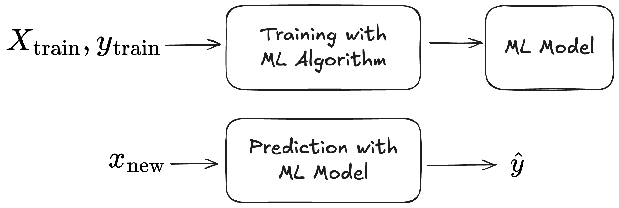
The first step towards a setup where we pre-train and move from train-then-predict to in-context learning is to conceptually wrap training and prediction into one function. This function accepts the triplet of training features, training labels, and the new data point and outputs the prediction. This is even something we could achieve with traditional ML approaches: Technically, we could wrap, say, both training and prediction of a random forest into the same function call.

Combining training and prediction in one function.

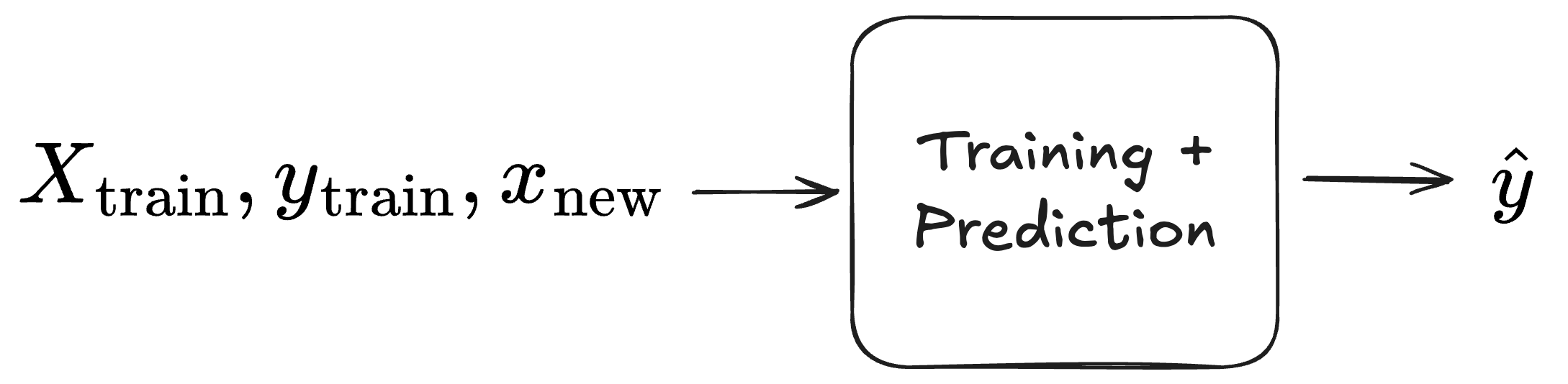
Note that this is not the same as in-context learning. But conceptually, it brings us closer to pre-training and in-context learning. If we see the model training simply as a nuisance, we can reframe our initial problem of wanting to know y from x given a model: We want a function that outputs a prediction, given the data point’s features, the training dataset, and the labels of the training dataset.

Let’s add one more thing to the wish list: Instead of predicting y, let’s predict the distribution p(y). If we have a model that not only predicts the expected value or some other aspect of p(y), but also gives us the entire distribution, we get a lot of utility for free, like quantile regression, uncertainty quantification, and outlier detection.

In mathematical terms, we would love to have the following:

\(p(y|x_{\text{new}}, X_{\text{train}}, y_{\text{train}})\)

In Bayesian terms, this is the posterior predictive distribution. Recognizing this allows us to do some Bayesian magic. Well, it’s actually just bits of probability theory, so don’t fear reading on.

Using Bayes to sneak in pre-training

We will use a bit of probability theory to define the posterior predictive distribution for a given dataset and data point to involve other training tasks (based on the PFN paper).

We start with the posterior predictive distribution:

\(p(y|x_{\text{new}},X_{\text{train}}, y_{\text{train}})\)

Using the law of total probability, we can insert a latent variable φ that represents the underlying supervised machine learning task:

\(p(y|x_{\text{new}},X_{\text{train}}, y_{\text{train}}) = \int_{\phi} p(y|x_{\text{new}},\phi) p(\phi|X_{\text{train}}, y_{\text{train}})d\phi\)

You might have noticed that we “lost” X_train and y_train in the first term, but this is because y is conditionally independent of the training data when we condition on the task φ, because the task fully specifies the data generation.

The last term, the posterior of φ given the data, is a bit awkward to estimate or think about. We can get rid of it with Bayes theorem, which says that p(A|B) = p(B|A)p(A)/p(B), drop the denominator, and get the following formula:

\(p(y|x_{\text{new}},X_{\text{train}}, y_{\text{train}}) \propto \int_{\phi} p(y|x_{\text{new}},\phi) p(X_{\text{train}}, y_{\text{train}}|\phi) p(\phi)d\phi\)

This formula of the posterior predictive distribution is the theoretical foundation of tabular foundation models like TabPFN.

So let’s distinguish the different terms:

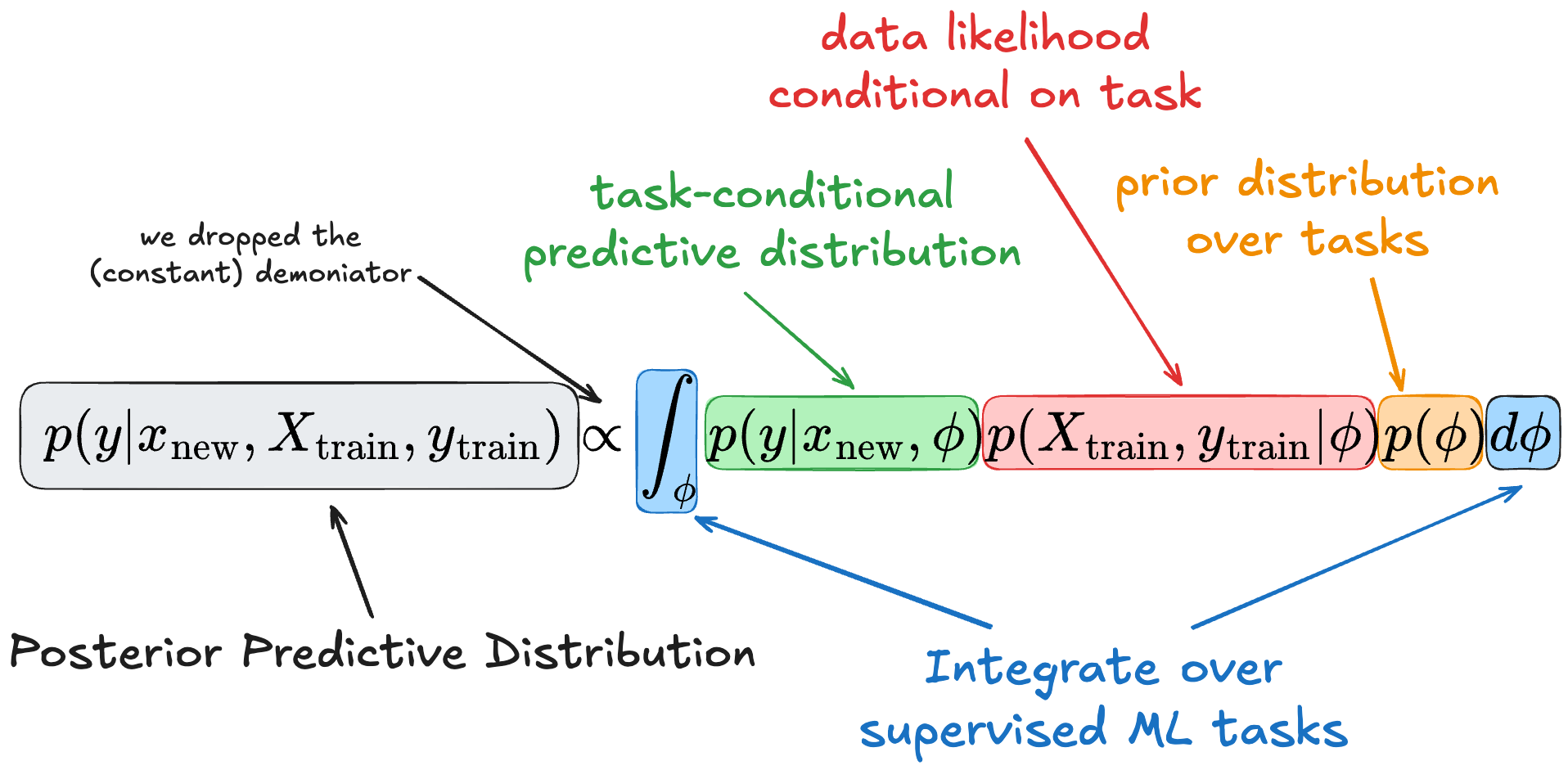
• The predictive posterior distribution of our target y, given its features x_new and a context dataset (aka training dataset), requires integrating over (latent) tasks.

• This integration over tasks has three components:

  • A prior probability p(φ) of tasks: this tells us how likely the task we are integrating over is.

  • Likelihood of the training given the task φ: this tells us how likely the observed dataset is given the task we are integrating over.

  • Probability of y given its features and the task φ: this gives us the probability of y given the feature vector and conditional on the task.

• Intuition: we marginalize over all possible latent tasks φ:, weighting the prediction p(y|x,φ) by how plausible φ is given the prior and how plausible the observed data is given φ.

Models like TabPFN approximate this posterior predictive distribution (PPD). However, it’s not done by modeling the components of the equation individually, but they take a different approach.

Task prior, synthetic data & transformers: ingredients to approximate the PPD

Here is how prior-data fitted networks (PFNs) such as TabPFN work:

• First, define a data-generating process from which one can sample tasks φ. More concretely, one way to do this is by defining a function that produces structural causal models with a different number of nodes and relations between the nodes. This essentially defines an implicit prior p(φ) from which one can sample tasks φ. Note that no explicit definition of p(φ) is needed. It’s just a generator that produces samples φ; p(φ) is implicitly defined by this process.

• Based on such a structural causal model, one can sample labelled datasets. I’ll go more into detail about how this works in a future post. This part basically gives us a way to sample from p(X_train, y_train | φ).

• The third ingredient is a transformer architecture adapted to tabular data that processes the entire dataset (training points together with the query point) in a single forward pass. Self-attention operates across rows (data points) and columns (features), allowing the model to condition predictions on both other samples and feature relationships. This enables in-context learning: rather than updating parameters, the model infers the task and its inductive biases from the provided dataset. This attention-based model, trained on millions of synthetic datasets, is transferable across tabular problems.

PFNs are a general framework in which one specifies a prior over data-generating processes. For pre-training tabular foundation models, this prior is specifically instantiated for tabular data. TFMs such as TabPFN and TabICL differ in their priors, architectural choices of the transformer-based network, and in pre- and post-processing steps, while sharing the same underlying PFN principle.

Next week, we are going deeper into the architecture of TabPFN (probably v2).