Improve Post-Hoc Interpretation By Leveraging Background Data

Model-agnostic interpretation methods like PDP and SHAP require data for estimation.

Now you could treat that simply as a nuisance, something to be dealt with like brushing your teeth every day.

But in this post I want you to try out a different view of this data. Not just the technical “estimation” view. But to view the data used for estimation as the background data. Because the background data is a surprisingly flexible part of your analysis which allows you to be creative and insightful.

Let’s dive in.

Example: Partial Dependence Plot

The partial dependence plot describes how the prediction changes, on average, when one of the features changes. The following plot is based on a model that predicts bike rentals from weather and other features. The plot shows the PDP for temperature.

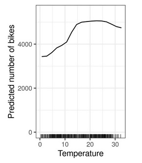
Interpretation example: The predicted number of rented bikes is, on average, 4500 when the temperature is 20 degrees Celsius (68 Fahrenheit). We can see a trend that the warmer the temperature, the more bikes are rented. This effect levels off at around 15 degrees Celsius and for very hot temperatures the bike rentals drop a bit.

To compute a point of this PDP, for example at 20 degrees, we take the 20 degrees and replace all temperatures in the background dataset with 20 degrees, get the predictions, and average them. Now you can already see how the background data comes into play: Whatever we choose as background data influences for which data points we get predictions and therefore what the interpretation is. And this data can be different from the training data. At least we have the option to pick a different dataset.

So we could also, instead of using all data points for computing the PDP, only get the data points for summer and compute a PDP for the effect of temperature on rented bikes only in summer. Or we can split the data by season and plot all four season-PDPs side-by-side.

Splitting the data into groups and plotting the PDPs in each group was also the idea behind one of our papers: A recurring problem of model-agnostic interpretation methods is correlated features. And by finding groups in which the feature is less correlated with others, we can reduce correlation.

4 Partial Dependence plots showing the effect of temperature on rented bikes. Each PDP is estimated with a subset of the data, automatically split by the season and humidity features. For winter, spring, and fall, higher temperatures are associated with more bike rides. In humid summer, the temperature has no effect. In dry summers the temperature even has a slight negative effect. PDPs are plotted as boxplots to show where the mass of the data lies.

Let’s look at the partial dependence plot based on its definition with random variables. It’s defined as:

\(PDP_j(z) = \mathbb{E}_X[f(X_j = z, X_{-j})] = \int f(X_j = z, X_{-j}) \mathbb{P}(X_j=z, X_{-j})dX_{-j}\)

Let’s break this down. This formula describes how to compute the partial dependence plot at a certain value of feature X_j (here argument z). We divide our features into the j-th feature and the rest (-j). Then we condition on X_j having value z and take the expectation over the data X_{-j} which boils down to an integral.

It’s simpler if you look at how the partial dependence plot is actually estimated.

\(\widehat{PDP}_j(z) = \frac{1}{n} \sum_{i=1}^n f(z, x_{-j}^{(i)})\)

So this is a simple sum over n data points where we forcefully replaced X_j with value z.

Usually, you would just pick training or test data to sum over and compute the PDP. But there’s no law that prohibits you from using other data or subsets thereof. Think of the data as the background data. By cleverly picking the background data, the simple PDP becomes a much more powerful tool because suddenly you can answer a lot more questions.

Some examples of what you can do by leveraging the background data:

• Simulate a distribution shift and get the PDP for the new data

• Analyze how the feature effects differ in different groups of the data

• Explore feature interactions by splitting data by another feature and plotting the PDPs side-by-side

• Reducing the correlation problem by splitting the data so that the feature is less correlated with other features

• Explore counterfactual scenarios: Set the background data to a specific scenario

• Evaluate the stability of the model predictions: By setting the background data to more extreme values, you can study how robust the model is.

The background data can also be used to do mischievous things, like adversarially changing the interpretation. Here is an example of a paper where the authors worked with a heart disease classification model. The PDP for age was changed to show a negative effect by changing the background data. The manipulated background data even showed roughly the same marginal distribution as the original data, but the PDP effect was inverted. The perturbation of the data was adversarial, so intentionally created to change the PDP. So don’t fear that this will just happen randomly in your data.

In blue: the original PDP showing risk increase with age. In red: the manipulated PDP showing a decrease with age. Source: DO NOT EXPLAIN WITHOUT CONTEXT: ADDRESSING THE BLIND SPOT OF MODEL EXPLANATIONS by Woźnica et al (2021)

Beyond PDP

Most model-agnostic methods rely on background data. Here are a few more examples:

• Shapley values for explaining predictions: The “absence” of a feature value is simulated by drawing values from the background data

• Permutation feature importance: The information of a feature is destroyed by drawing a value from the background data

• Surrogate models need training data which can be seen as background data for their interpretation

• …

For these methods, you also have the power to improve your analysis by cleverly picking the background data.

For other model-agnostic interpretation methods, it really depends on the implementation. For example, counterfactual explanations have many different ways of being estimated. For some you need background data, but not for all.

Takeaway: Don’t see background data as a mere nuisance for estimation, but utilize it to your advantage to create a more in-depth analysis.

P.S.: I’m working on a Shapley values book. Sign up here to get notified.