Old-School Interpretability for LLMs

SHAP Isn’t Dead

Mechanistic interpretability has taken most of the spotlight when it comes to the interpretation of LLMs. Unfortunately, except for some initial sparks, mechanistic interpretability hasn’t delivered. Especially not for users of large language models.

But what about the good old methods of interpreting machine learning models, like Shapley values and other methods that explain the outcome by attributing it to the inputs?

Explaining LLMs with such tools is a bit more complex than explaining, say, a random forest regressor on the California housing data, but it’s feasible.

In this post, I motivate how attribution methods for LLMs work.

An LLM is just a classifier

A large language model is a classifier. Given a sequence of tokens as input, it outputs a probability distribution over the vocabulary of tokens. Token vocabularies can be quite huge; for example, GPT-5 has a token vocabulary of size 200k.

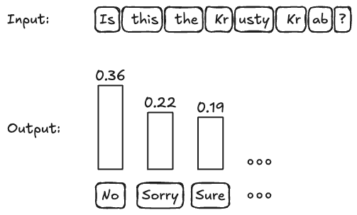
If we tokenize “Is this the Krusty Krab?”, we get [“Is”, “ this”, “ the”, “ Kr”, “usty”, “ Kr”, “ab”, “?”]. If you input this into an LLM, and you get a distribution over tokens, see the next figure. The “No” rightly gets the highest (=least negative) log probability of -1.017898440361023, which corresponds to a probability of ~36%.

LLMs accept a sequence of tokens as input and output a probability distribution for the tokens in the vocabulary.

That looks to me like a classic setup for perturbation-based explanation methods such as Shapley values, LIME, and counterfactual explanations. These methods manipulate the inputs and get new model predictions from which they compute the explanations. No knowledge about model internals, such as the architecture or weights, is needed.

Since we are in a multiclass setup, we have to pick one class beforehand. For example, we could create an explanation for the token “No”, which means picking its log probability as the explanation target.

Shapley values for next-token prediction

We could compute Shapley values for each input token: How much did they contribute towards the prediction of the token “No”, compared to a baseline? To understand the baseline, here is a quick idea of how Shapley values work: We compute how much each input feature (here: token) contributes to the prediction (here: log prob for token “No”) by computing its marginal contribution to many different coalitions of features. This requires turning features on and off, depending on whether they are in the coalition or not. When a token is “on,” we keep it unchanged in the input; We turn it “off” by replacing it with a (sampled) token or removing it from the text.

The Shapley values method produces one attribution value per input token. A positive value means that the token’s presence increased the log probability of the output, and a negative value means that it decreased the log probability. Always compared to the baseline (e.g., where we delete “off”-tokens).

If you want to learn more about Shapley values, read the Shapley Values chapter in my Interpretable ML book, or for the full experience, get my book Interpreting Machine Learning Models with SHAP.

We need log probabilities for explanations (kind of)

All these computations assumed that we have full access to the log probabilities of the model. For open source models, not a problem. For closed models hiding behind an API, it’s tricky. Some closed models like GPT-5 and Claude don’t provide log probs at all. Others, like GPT-4 or Gemini, only provide the top-something log probabilities.

We can, however, compute many of the explanation methods directly using a fixed class, so we can still use Shapley values and the like for closed models that don’t provide log probabilities. However, this means only changes in the most likely token will be noticed, which should make the explanations much rougher. Especially if you are looking to create explanations not for the top token, but for another one.

And then we get the bill

The larger issue is computational cost. To compute Shapley values, you have to make at least a couple of hundred calls to the model. The number depends on the input text size, the baseline replacement strategy, and the variance of the LLM output.

Again, open source LLMs have a clear advantage here, at least when self-hosting:

• Each call is typically cheaper than paying for API-based models. At least if self-hosted.

• If you have access to the gradients, you can use a model-specific implementation of Shapley values (GradientExplainer), which is faster than the model-agnostic explainer.

But it gets even more expensive …

One token? Who cares? Explain the entire output.

So far, we’ve talked about explaining a 1-token prediction. But we probably care more about explaining an entire output text.

Example of input and output

If the output text has 6 tokens, the model makes 6 predictions. If we still wanted to compute attributions with LIME or Shapley values, we would get 8 x 6 = 48 attribution values, one for each combination of input and output token.

The combinatorial issue of attribution methods.

We also have to approach this sequentially: First, compute the Shapley values for “No”, then concatenate “No” with the input, and compute the Shapley values for “,” (but without perturbing the “No” in the input.) And so on. This token-to-token attribution gives you a table of attributions. You can, for example, use software like Captum to achieve this.

Example of full token-to-token attribution with Shapley values. Source: https://captum.ai/tutorials/Llama2_LLM_Attribution

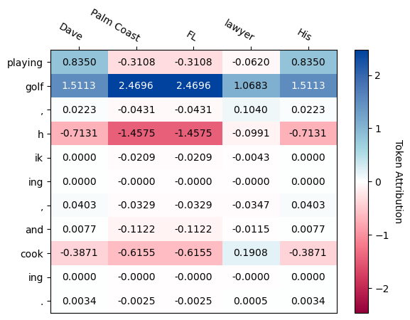
If you check the figure above closely, you might spot a deviation from the strict token-to-token explainability. “Palm Coast” is a combination of 3 tokens, but appears only as 1 input. That’s something you can do with perturbation-based methods: simply group features and switch them on and off simultaneously. The Captum tutorial from which the image is from also shows an alternative to removing tokens that are “switched off”: For example, place names like “Palm Beach” are replaced with other place names. This fixes the implausible-sentence problem but also changes the interpretation.

By playing around with the replacement tokens, we can get very creative. For example, depending on the use case, you might group entire input sentences or even paragraphs to compute their joint impact on the output. The choice of replacement snippets allows you to steer the model interpretation. I used a similar strategy to win in a machine learning competition that was focused on interpretability, the water supply forecasting competition (this was on tabular data, though).

All in all, we can definitely use good old interpretability methods for explaining LLM outputs. It can get expensive and a bit tricky, especially with closed LLMs, but it’s feasible.