
Building Block View of ML
The interesting bits from the book I quit

Inspired by the modular nature of neural networks, can we see all machine learning algorithms through the lens of building blocks?
Let’s deconstruct machine learning.
We are just looking for a function
Machine learning can be described in terms of three building blocks1:
Learning = Representation + Evaluation + Optimization
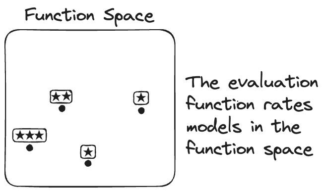
Our goal: we want the computer to learn a function from data.2
The problem: There are infinitely many functions in the function space. The function space contains all possible functions one could think of that match our task. For example, for regression with 10 features, the function space contains all functions that map the 10 features to 1 outcome.
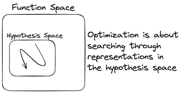
By picking a representation, we can restrict that function space to a smaller hypothesis space.
For example, the hypothesis space could be binary decision trees or linear models. These are still infinite spaces, but they are the manageable kind of infinite.

But before the computer can start searching through the hypothesis space, we need the building block of evaluation. Evaluation helps us distinguish good from bad functions/models. Measures such as precision and recall, for example, can distinguish good from bad functions for classifying data.
With representation and evaluation in hand, the only part missing is a procedure to search through representations in the hypothesis space. Building blocks of such optimization procedures are gradient descent, beam search, exhaustive search, the EM-algorithm, and many more. They tell the computer how to traverse the hypothesis space to come up with a good function.
For example, we can deconstruct linear regression in the following way:
linear regression = weight vector (representation) + mean squared error (evaluation) + gradient descent (optimization)
The four building blocks of representation
When it comes to representation, four fundamental building blocks make up most of modern machine learning:
Models can store patterns as data points, and apply them by retrieving the labels of the closest ones (kNN, k-means, kernel methods, …)
Models can store patterns as if-then rules (RIPPER, Random Forest, xgboost, CART, …) and apply them by matching features with conditions.
Models can store patterns as weight vectors and apply them via the dot product (linear regression, convolutional neural networks, logistic regression, …)
Models can store patterns as distributions and apply them through probability calculations (Naive Bayes, generalized linear models, …)
Let’s explore these different representations.
Representation with points
Machine learning models may store “learned” patterns as points. To predict a new data point, retrieve the labels of the closest “stored” points. Point-based ML models have an intuitive geometric interpretation: The features define coordinates in a space, where each feature is a dimension. New data points are then defined by their positions in that space, relative to the stored points. Closer points (neighbors) are deemed relevant for predictions of the new data points.
The most famous point-based ML algorithm is the k-nearest neighbor algorithm, which uses the data points from the training data as representation.
. A new data point is show and the closest neighbor is highlighted.")
Point-based models need two building blocks:
A set of data points as storage
A distance function (e.g. L2, L1, gower distance, …)
Optimization-wise, kNN is weird, since the algorithm doesn’t have a training step. There is still optimization involved (if you want to call it that), but it’s at prediction time, and it’s an easy optimization problem: find the stored data point with the smallest distance to the new data point.
Clusters and other prototypes are also point-based representations
There’s no law against creating new points for representation. Clustering algorithms, for example, often use cluster centers for representation. Clusters are typically newly created points, an example being k-means.

Cluster centers belong to the broader category of prototypes, which are points that describe aspects of the data distribution and can serve as building blocks to represent machine learning models.
Creating points introduces a new optimization problem, and we can’t rely on “lazy learning” as with k-nearest neighbors. Many prototype-based ML algorithms use alternating optimization (e.g, Lloyd’s algorithm, EM-algorithm), alternating between optimizing the coordinates of the prototypes and another step, typically the assignment of data points to the prototypes.
Represent models with IF-THEN rules
A simple yet effective way to represent data patterns is using IF-THEN rules. Like:
IF (garden=Yes AND apartment_size>100) THEN rent=high.
To predict, check the IF statement, and if the conditions match the features of the new data point, use the THEN part as the prediction. A decision rule can have multiple conditions connected with AND statements.
A decision rule has a nice geometrical interpretation: the conditions of a rule carve out a partition in the feature space — a rectangle if it’s 2 features, a cube if it’s 3, and so on (assuming we have min and max values for each feature).

The optimization problem of learning a rule is combinatorial: Imagine we have three binary features. Then there are 27 possible rules. That’s because a binary feature can be `True`, `False`, or not used at all by the rule; that’s, in total, 3^3=27 possible rules. For a few features, exhaustive search is possible: try all combinations and pick the best one. But with more features, exhaustive search becomes unfeasible. Even worse when we also consider continuous and multi-valued features.
The most common approach in rule learning is greedy, bottom-up search. Start with an empty rule (no IF conditions), try each possible condition, and add the one that works best to the rule. Continue adding conditions to the IF, connected with AND, until a stop criterion is reached. A bit oversimplified, but most rule learning algorithms are just variants of this.
Combine multiple rules into lists and trees
A single rule is typically just a building block and not yet a full model. To get a full model, we need to combine multiple rules into a rule set. But this introduces two problems that need to be addressed:
No rule applies: There may be data points for which no rule applies. The easy fix is to add a default rule that applies if no other rule matches.
Overlapping rules: Two or more rules may apply to the same data point. To resolve this, the model needs a resolution strategy like majority vote, or the model representation needs to be restricted to only allow for non-overlapping rules.
There are two rule-based representations that fix the problem of overlapping rules by simply avoiding them: lists and trees.
A decision list is an ordered set. To predict, start with the first rule in the list. If it applies, the prediction is the respective THEN part of the first rule, and you are done. If not, proceed to the second rule and so on. Constructing such a set (=optimization) is typically done with the covering algorithm. Pick any algorithm to learn individual rules, and apply it to the data. Remove all training data covered by the rule conditions. Train the next rule on the remaining training data. Remove covered data. Repeat until no data is left or some other stopping criterion is reached.

The second antidote to overlapping rules: the decision tree. At first glance, it doesn’t seem like decision trees are decision rules, but we can always deconstruct a decision tree into a set of disjunct decision rules, where each leaf becomes one rule. Trees are grown hierarchically instead of sequentially. Their optimization is adapted to that hierarchical nature, but we still typically start with zero features and add one at a time (=greedy).

Ensembling Trees
Today’s state-of-the-art ML algorithms for tabular data use decision trees as a building block. To be more exact, they use ensembles (=sets) of trees. Ironically, this reintroduces the problem of overlapping predictions, but this time it’s a feature, not a bug. The motivation behind ensembles is to leverage the “wisdom of the crowd” effect.
Wisdom of the crowds requires decision trees trying to predict the same thing (e.g., predict rent), but being sufficiently different from each other. Two methods to learn diverse trees are established:
Bagging: Draw with replacement from the training data to create a dataset of the same size. Train a tree on this data. Repeat sampling and training a couple of times to get different trees. The random forest algorithm relies on this strategy.
Boosting: Learn trees iteratively on the errors of the trees before. Only the first tree is trained on the original target. Many machine learning algorithms use this strategy: xgboost, catboost, lightgbm, …
Bagging and boosting are different building blocks of optimization, but they create models that have the same representation, namely, tree ensembles, which consist of a set of trees and a resolution strategy.

Weight Vectors
The humble weight vector is the building block for models ranging from a simple linear model to transformer-based large language models. The basic idea: Store weights in a vector and apply them to the (intermediate) features by multiplying each weight by its corresponding feature and summing up the results. In short, this operation is called the dot product.
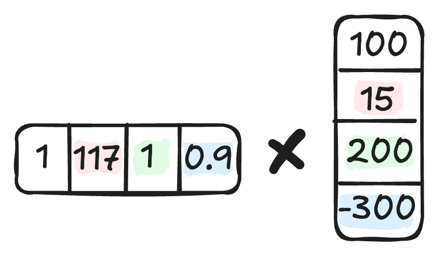
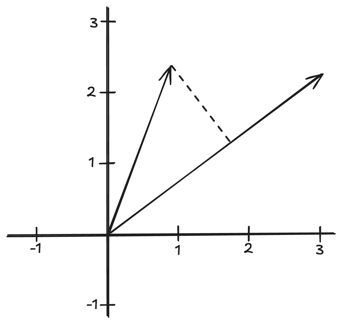
This building block, too, has a geometric interpretation. The dot product measures the alignment between the feature vector and the weight vector, multiplied by their lengths.
To learn weight-based models, we typically use gradient descent. This optimization method, or rather, family of optimization methods, has become a central building block for more complex models.
Nonlinear functions
Before we can build anything more complex with weight vectors, we need nonlinearity. If we sequentially chain dot products, we end up with a model that we can represent with a single weight vector, so nothing is won compared to the linear model. The path to more complex models is sequentially combining dot products with nonlinear functions.
Nonlinearity as a building block also has another use in machine learning: It allows us to change the space of a feature (or target). For example, the logistic function allows us to turn a linear model into one that outputs probabilities (or, at least, numbers between 0 and 1).
Let’s stack some weight vectors
Using weight vectors and nonlinear functions as building blocks, we can build neural networks. It’s not just the feedforward networks, but most neural network layers are creative applications of the dot products: convolutional layer, attention layer, …
Each dot product + nonlinearity can be seen as a feature transformation. Putting them in parallel (= having multiple neurons in a layer) means computing multiple features in parallel. Chaining them sequentially means transforming the feature space and is what ultimately allows a neural network to learn more complex functions.
Even though such architectures can become very complex, we can still train them with gradient descent.
Distributions
Distributions store patterns in probabilistic form, and we apply them through probability calculations, especially the conditional expectation. This building block requires us to see features and targets as random variables. Sometimes it also means introducing additional latent variables. All these random variables have a distribution.

We can leverage distributions to make predictions by expressing predictions as conditional distributions: Given we already know the features, what is the distribution of the target? This doesn’t give us a single answer, but a distribution — basically a weighted range of answers. To boil it down to a single prediction, we can summarize the distribution with the expected value. This predictive view of distributions is narrow, as distributions allow us to model the full range of uncertainty of the prediction.
To represent our target in terms of a conditional distribution, there are two typical options:
Take a closed-form mathematical distribution, like the Gaussian distribution, and express a parameter of that distribution in terms of the features.
Build a distribution from smaller building blocks, such as splines, and link their weights to the features.
Learning distributions is then all about maximizing the likelihood of the data by changing the parameters. Also, evaluation is based on likelihoods, which is a bit circular, as we can only compare likelihoods within the same family of distributions. Anyways, in a predictive setup, we can compare predictive performance, like MSE or F1.
Some distribution-based ML models “collapse” to a weight-based representation. For example, we can express the linear regression model as the conditional Gaussian distribution of the target given the features, but we only need to store a weight vector.
That’s it! Well, there are many more building blocks, like all the evaluation metrics, data splitting and resampling, mixing building blocks, and so on. But enough for today, at least.
Based on: Domingos, Pedro. “A few useful things to know about machine learning.” Communications of the ACM 55.10 (2012): 78-87.
There are exceptions, which are mostly found in unsupervised learning: ML models produced by, for example, DBSCAN and hierarchical clustering produce patterns, but not functions that we can use on new data.