Machine learning interpretability from first principles
Understand interpretation methods via functional decomposition
There are hundreds, probably thousands of methods to interpret machine learning models. SHAP, permutation feature importance, partial dependence plots, counterfactual explanations, SAGE, … you name it. It’s confusing, especially if you get started.
Learning method after method can make you miss the forest for the trees. There are fundamental principles that interpretation methods rely on:
A model is just a mathematical function
The function can be broken down into simpler parts
Interpretation methods address the behavior of these parts
This post gives you the keys to understanding most machine learning interpretation methods.
Principle #1: A model is a function
However complex machine learning can be, the model itself is just a mathematical function.
The model f is a function that accepts the p-dimensional feature vector x as input and produces a 1-dimensional prediction.1
Our goal is to understand this function.
Writing the model function down sucks
Can we write this function down for any ML model?
For a linear model, we can.
For a random forest or a neural network? Not really.
2 problems:
Nobody gives us the formula. For example, fitting a model with sklearn produces an algorithmical version of the formula, but not a mathematical expression.
We can write down the formula for complex models, IN THEORY. It would be an ugly exercise: A random forest with 500 trees and each tree around 10 terminal nodes would result in a weighted average of 5000 nodes with lots of indicator functions to express the tree splits. Can’t recommend it.
And even if you would extract the formula, it would be all convoluted and non-interpretable for most prediction functions: We can’t read out the importance of the features, we can’t see how changing one of the features changes the prediction, etc.
Time for a different approach.
Principle #2: Any function can be broken down into simpler parts
We need an interpretable representation of the formula of our model.
Let’s say we have 3 features.
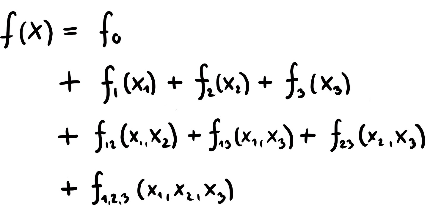
What would you say if we could represent our model function in the following way?
This formula decomposes the model into components with different dimensions and features.
An intercept that depends on no feature at all
The main effects are functions that only depend on one feature at a time
The interactions are functions that reflect the shared effect of 2 or more features
If we could decompose our prediction function like this, the interpretability of our model would be much better: It’s an additive formula, so we can interpret each component in isolation. For example, we can understand f1 as the effect of feature X1 individually and f12 as the additional interaction effect of X1 and X2.
But can we actually represent our model in such a way?
The good news: We can decompose any function in this way. It’s called functional decomposition (among other names). It’s not only used in interpretable machine learning but you find it in statistics, sensitivity analysis, and many other fields.
The bad news: Decomposing your model in such a way is often unfeasible, except if you have simple models with few features or constrain the formula by forcing many components to be zero. Also, the decomposition needs further assumptions that make the decomposition uniquely computable. For example, without further assumptions f12 could fully “absorb” f1 and f2, so that f1 and f2 would be zero. Read more in this chapter about functional decomposition.
Principle #3: Interpretation methods address the behavior of these components
We aren’t using functional decomposition as a technical solution, but as a mental model to understand machine learning interpretation methods.
When you think about a machine learning model (for tabular data), I want you to have the following image in your mind:
This decomposition is our starting point. Most model-agnostic techniques describe or aggregate these components and that gives us a principled way to discuss and understand all the different methods.
Permutation Feature Importance
Permutation feature importance (PFI) is probably the most simple interpretation method to explain.
The goal of PFI is to quantify how important a feature is for correct predictions. Measure the performance of the model on test data, permute one of the features, and measure the performance again. The larger the drop in performance, the more important the feature was.
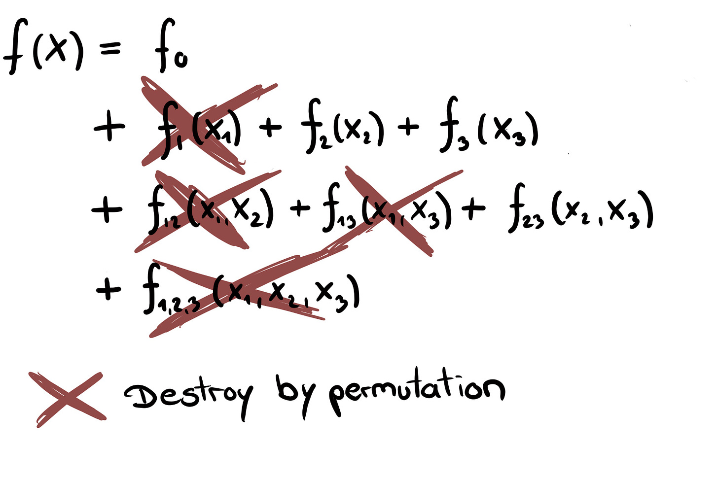
Let’s understand permutation feature importance via decomposition. Let’s say we permute feature X1. All the components that have an X1 in them are affected by the shuffling:
“Destroying” doesn’t mean setting the components to zero but the permutation has the effect of averaging over the distribution of X1, which can be interpreted as destroying the information. All other components without X1 in them remain untouched. In the 3-feature example, the components f1, f12, f13, and f123 are affected. This tells us that PFI isn’t the importance of the feature in isolation, but includes all its interactions.
SHAP values
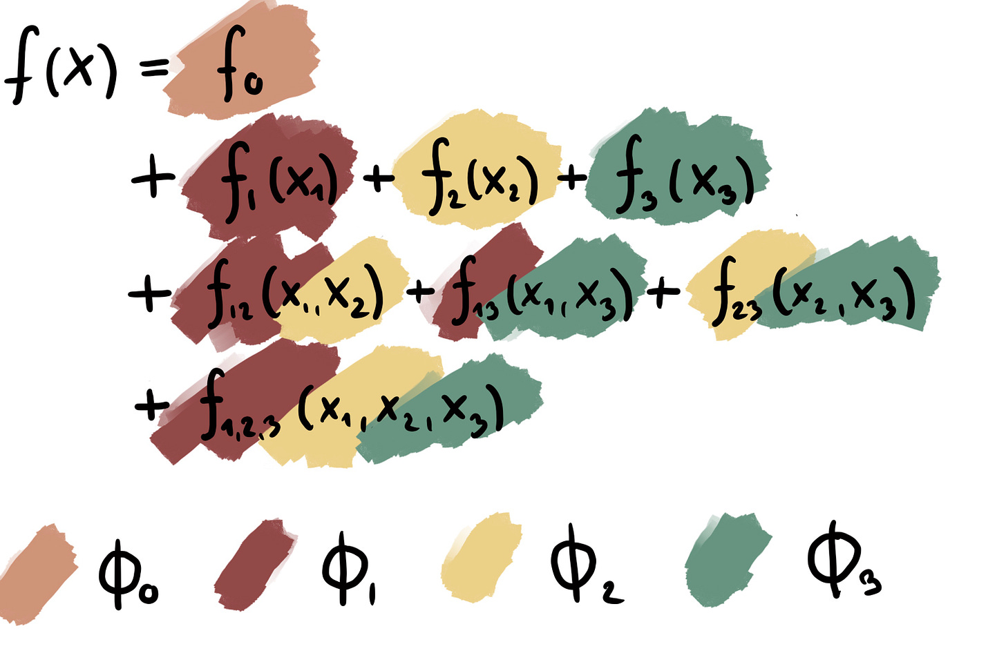
SHAP, an explainable AI technique, is a so-called attribution method that fairly attributes the prediction among the features so that the prediction is presented as a sum. Each feature gets a SHAP value, usually noted with the Greek letter phi ɸ, so that a prediction is explained like this:
While it looks similar to a decomposition, it’s an attribution: SHAP values aren’t functions but values that add up to a particular prediction.
But we can still use the decomposition to reason about SHAP values.
The SHAP attribution doesn’t have ɸ’s for the interactions, so what happens to these terms? For SHAP, the interactions are fairly split among the features so that each SHAP value is a mix of the main effect and all the feature’s interactions.
Accumulated Local Effect Plots
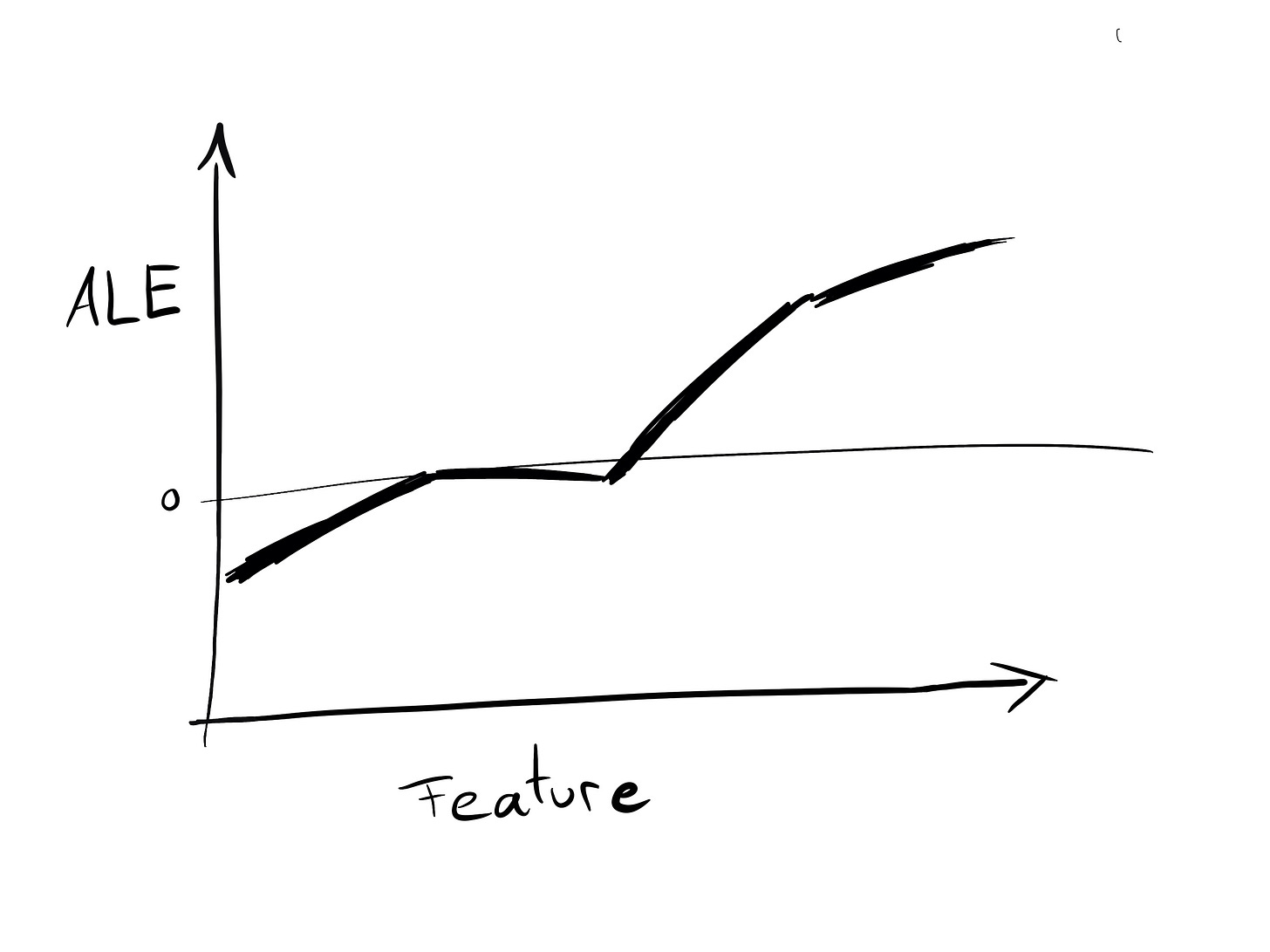
Accumulated Local Effects (ALE) describe how changing a feature changes the prediction.
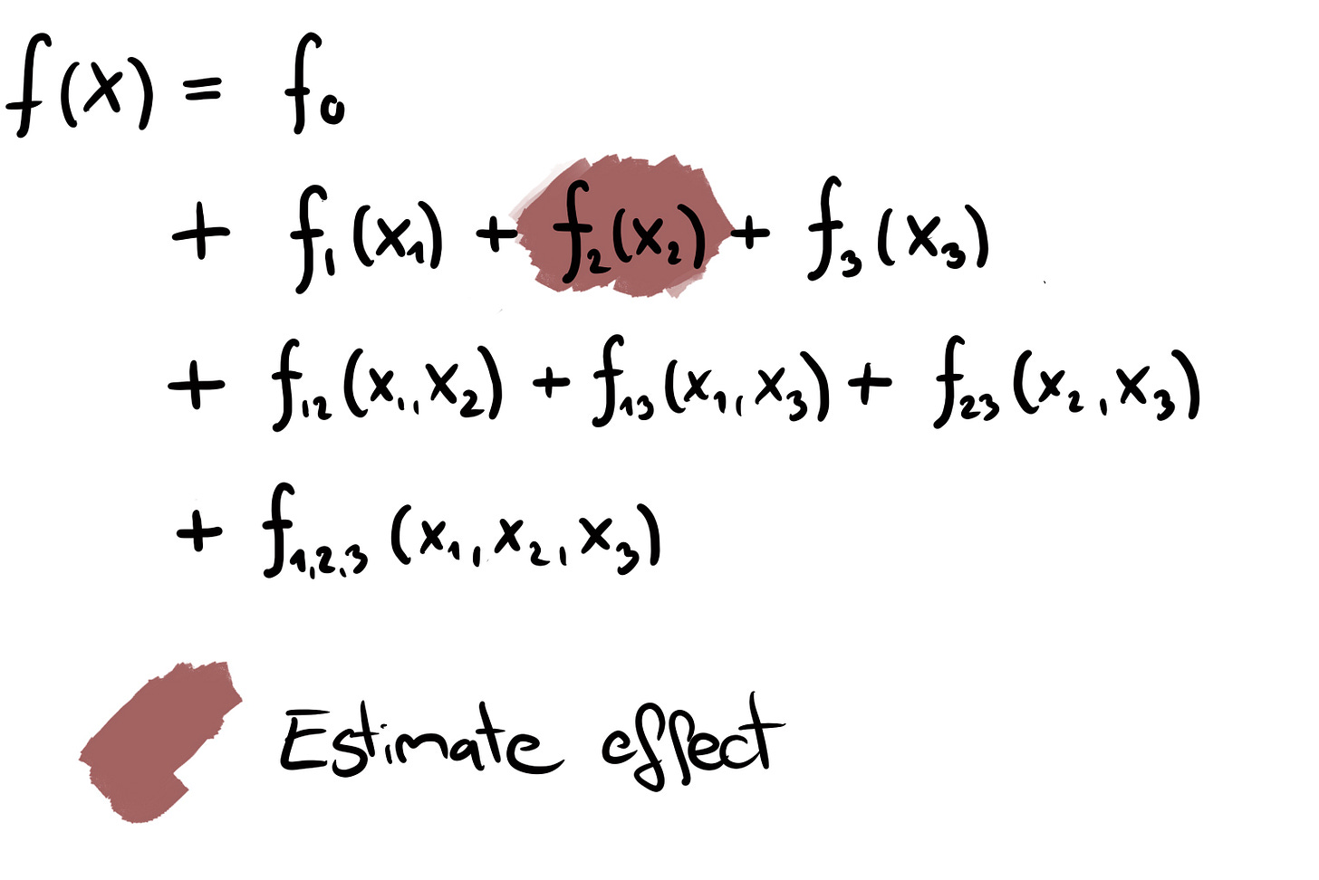
ALE is not only an effect plot, but also a valid method for functional decomposition! That means when we compute the ALE for X2, it represents an estimate of the component f2. To understand the assumptions that go into the ALE decomposition, read the chapter in Interpretable Machine Learning about ALE.
This list could go on but the post would become too long. If there are interpretation methods for which you’d be interested in the “decomposition view”, let me know in the comments.
Some models produce multiple outputs, like multi-class classification, but we’ll focus on 1D outputs. And often times they can be reduced to 1D, or have to anyways for interpretation. For example for interpreting multi-class classifiers, you usually look at just one class at a time.


This is so helpful. Please give this view for partial dependency plots (PDP) as well. Also closely related are partial effect plots (PEP); I don't know if the intuition is different for these two. (Here's a brief explanation of the difference between the two: https://stats.stackexchange.com/questions/371439/partial-effects-plots-vs-partial-dependence-plots-for-random-forests). PEP seems to be more popular with those who model with the statistical mindset whereas PDP is more popular with the machine learning mindset.
This is a beautifully intuitive explanation. However, I feel you left us hanging with ALE, which is precisely what interests me the most. So, I understand that for x2, ALE gives only the f_2(x2) component and nothing else. But then what about the interactions? Am I correct to understand that
* the simple ALE x2 score does not incorporate anything whatsoever of the x2 interactions; and
* the ALE interactions x1_x2 and x2_x3 map directly to the functional decompositions of f_12(x1,x2) and f_23(x2,x3)?
(I won't comment for now on the three-way interaction, since that is not yet well-developed for ALE).