
How to make Tabular Foundation Model inference faster
GPU, KV caching, context optimization, and other inference tricks

The greatest bottleneck with tabular foundation models: Prediction, aka inference, is slow.
This post is a collection of tips and tricks to make tabular foundation models much faster. BUT! There is always a price to pay. And you must decide on that bargain. Some improvements are cheaper, some are more expensive.
If you haven’t heard about tabular foundation models, check out my series on TFMs:

Let’s start with a “cheap” option for improving the prediction time of tabular foundation models.
Pick a faster foundation model (currently TabICL)
There has been a flurry of new models in the TFM space. Not all have the same inference time. It may be worth comparing the speed of multiple TFMs.
Which one is the fastest TFM? This is subject to rapid changes, but here is a quick first idea, based on TabArena. If you don’t know TabArena, check out my post.

The following leaderboard excerpt shows that TabICLv2 is, on average, the fastest TFM, but not the most performant. The best-performing model is TabPFN-2.6, with a slightly better Elo than TabICLv2.
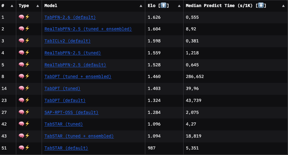
However, results from TabArena are averages (or medians) and therefore just rough pointers. You won’t know which TFM performs best on your task until you try.
I compared the prediction time of TabPFN and TabICL on the UCI breast cancer dataset: Switching from TabPFN to TabICL reduces inference time by ~14% (TabICL: 0.42 seconds; TabPFN: 0.49 seconds). TabICL (acc: 0.98, logloss: 0.067) even slightly outperforms TabPFN (acc: 0.97, logloss: 0.087) on this data.
Use a GPU
Tabular foundation models are neural-network-based and are much faster on a GPU than on a CPU. If you are GPU-poor like me, this sucks, as it requires getting access to a GPU. With boosted trees and other classic machine learning algorithms, I was able to run most projects on my good old MacBook M1. With tabular foundation models, a GPU is much, much more performant. Switching from CPU to GPU is one of the best levers to improve prediction time.
To give you an idea: Classifying the breast cancer dataset on a CPU with TabICL (on Google Colab) took ~15 seconds. Switching to GPU reduced that time to ~0.5 seconds, which is a 30x improvement.
Cache training representations
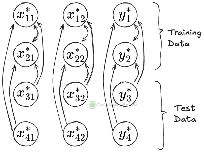
For each prediction call, tabular foundation models push the entire training data through the network. Let’s say you have two test sets for which you make predictions in two separate .predict() calls. For each of these calls, most computations are identical. That’s because the most compute-intensive parts are the transformer modules in the neural network. Here, training data can attend to training data, and test data can attend to training data. That first part, training-attends-training, is the same for each .predict() call, regardless of what the test data looks like.
A clear case for caching, right?
Super easy to do, here with TabICL:
clf = TabICLClassifier(kv_cache=True)
clf.fit(X_train, y_train)
clf.predict(X_test)
With caching, the .fit() call stores the training data computations in a key-value store. The .predict() step can now run faster since it only needs to make computations for the test data and can look up all the attention values for the training data.
For the breast cancer data, this reduces the .predict() time from 0.5 seconds to 0.09 seconds for TabICL.
But there is a catch. Two, actually.
First, caching costs memory. A lot of memory. According to the TabPFN 2.5 paper, 6.1 KB of GPU memory and 48.8 KB of CPU memory per cell of the training data. So, in our case, for a small dataset of 455 rows and 31 columns, which means 14105 cells, we already have 86 MB of GPU memory and 688 MB (~0.67 GB) of CPU memory. And that’s for a small dataset. That makes caching more realistic for small data or for reduced contexts. For TabICL, I haven’t found the memory numbers, but I suspect they will be in the same ballpark.
The second catch: While .predict() is faster, .fit() is accordingly slower. So if you do a single train/test split and call .predict() exactly once with the same context data, the KV caching will be useless. Use caching only with repeated .predict() calls and when you actually do have the memory.
Context Optimization
Models like TabICL scale with O(n^2m + nm^2). Assuming the number of features m is much smaller than the total number of rows n, and context data dominating n, then halving the context data size may almost mean a 4x reduction in compute time. Any strategy that reduces context size substantially improves speed.
Reducing the context size usually means lower predictive performance. The following chart shows how simple subsampling with different sample sizes of the context data affects predictive performance, in this case for the UCI wine quality dataset.
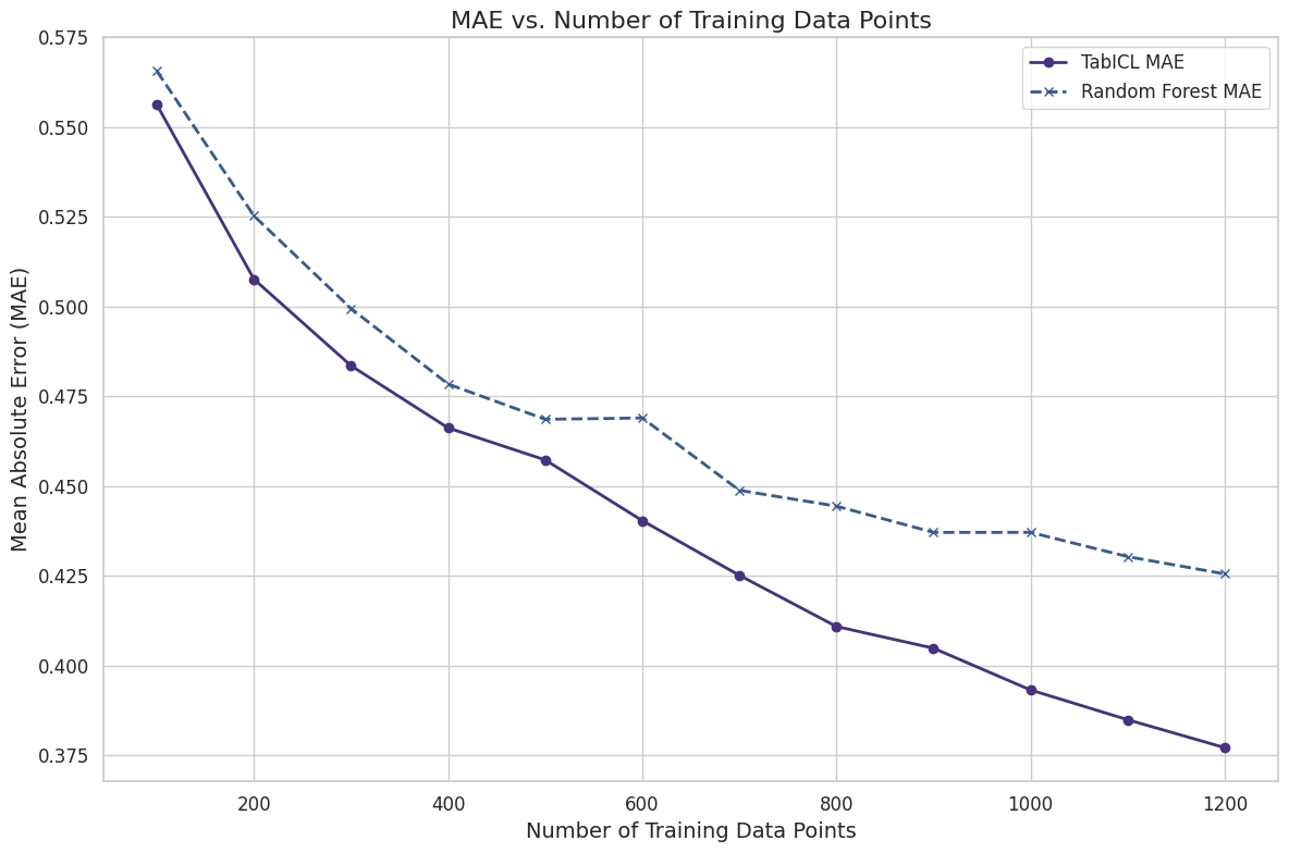
There are also smarter ways to reduce context size, such as a k-nearest neighbor-based approach and data/distribution distillation approaches.
More details on context optimization in this post:

Since TabICL’s runtime of O(n^2m + nm^2) is also quadratic in terms of the features, reducing the number of features is also an option, especially if you start out with lots of features. To reduce the number of features, we have the entire toolbox available, from dimensionality reduction to feature selection.
Reduce the ensemble size
When you call tfm.predict(), you get the result from multiple TFM calls with slightly different parameters. This has to do with the dependence of TFMs on the column order.
The default ensemble size is 8 (coming down from a whopping 32 in the first version of TabICL). Hiding in there is therefore an up to 8x speedup. The speedup is usually at the cost of reduced performance, but not always. In the case of the breast cancer dataset, we get with TabICL:
8 estimators: 0.42s and a logloss of 0.0671
4 estimators: 0.22s and a logloss of 0.0659
2 estimators: 0.11s and a logloss of 0.0760
1 estimator: 0.06s and a logloss of 0.0717
In this case, accuracy even stays the same between 8 and 1 estimators. Here, reducing the ensemble to 1 estimator is justified and gives us a huge speed improvement. For your own data, I recommend verifying whether an ensemble reduction brings speed improvements.
Train a surrogate model
You may distill a TFM into a surrogate model, like a tree ensemble or a multi-layer perceptron. The distillation approach can make sense if you do a lot of inference with fixed context/training data or run it on constrained devices. But you lose all the benefits of using TFMs in the first place, especially the flexibility in context used, embeddings, and so on. Especially if TFMs move into a multi-modal and relational direction, which I strongly suspect, this line will be much less relevant.
Key speed improvements for the impatient
Use a GPU.
Switch to a faster TFM.
If memory allows, use KV caching for repeated predictions with the same context.
Let optimizations compound: For example, GPU inference plus KV caching can improve prediction time by well over 100x.
Also: Scaling is a high priority for most TFM labs. I expect further improvements in architecture and inference tricks, which will bring down the .predict() time.
Very timely. Was just beginning to plan the process of context distillation, both for tabular and data quality reasons. Always find this to have useful insight!