
SHAP Interpretations Depend on Background Data — Here’s Why
Or why height doesn't matter in the NBA

Last week, I held my first-ever workshop on interpretable machine learning. One thing we explored was how the choice of reference or background data affects SHAP interpretations.
This aspect is often underappreciated—both as a potential pitfall in interpretation and as an opportunity. I previously wrote about the power of background data in other interpretation methods, but there is more to be said regarding SHAP.
Example: Wine Quality Prediction
To illustrate this, let's look at the wine dataset, where the goal is to predict wine quality based on physical and chemical features. I trained a random forest model, with each row representing a different wine. Then, I used SHAP to explain the predicted quality of a specific wine.

Initial Interpretation:
The selected wine has a predicted quality of 6.745, which is higher than the average predicted quality of 5.924.
The primary positive influence is its alcohol content (12%) which raised the prediction by +0.5 compared to the average prediction.

The Role of Background Data
Estimating Shapley values requires a background dataset for sampling. The key idea behind Shapley values is that features act as a "team," and the prediction is fairly distributed among them. The algorithm computes what predictions different coalitions (subsets of features) would receive. Since most ML models require all features to be filled in, missing values are sampled from the background data.
However, the background data is not just a technical necessity—it fundamentally changes how we interpret SHAP values.
New Background Data: To demonstrate this, I re-ran SHAP using a new background dataset consisting only of wines in the top alcohol quantile (>11.4%). The results were strikingly different:
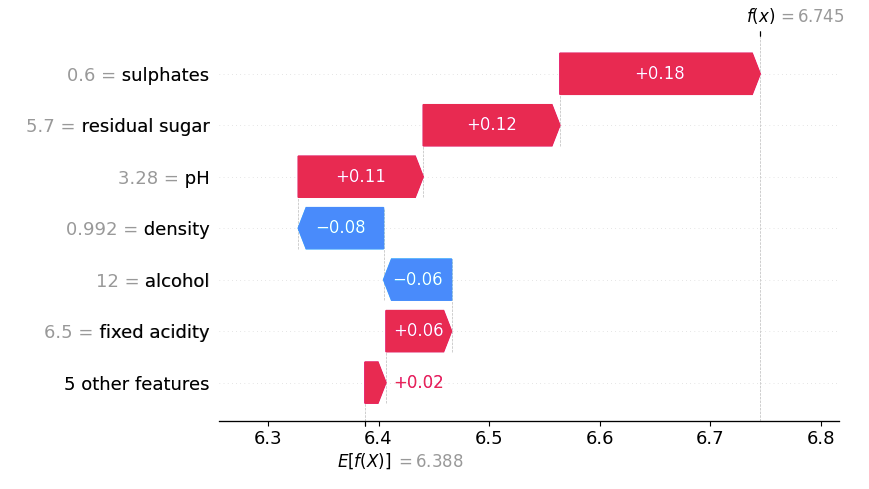
Previously, alcohol was the strongest positive influence. Now, it has a slight negative effect.
Sulphates became the most influential feature, whereas before it was only third.
The expected prediction E[f(X)] shifted to 6.388—higher than before because it’s now based only on high-alcohol wines. And on average, high-alcohol wines were rated higher in this dataset (and the random forest picked that up as well).
Why Does This Happen?
Conditioning on high-alcohol wines means alcohol is no longer a distinguishing factor. If we replace the alcohol level with a random value from the new background set, it will still be at least 11.4%, possibly even higher than 12%. Thus, alcohol no longer explains much variation.
A similar analogy can be found in basketball:
Height matters for performance when playing basketball.
But within the NBA, where most players are tall, height no longer explains performance differences.
This effect resembles biases like collider bias or selection bias, but labeling it as "bias" can be misleading. Whether it’s a problem depends on the purpose of the analysis. In some cases, restricting the background dataset to a specific subset is intentional and valid—such as when comparing a wine against only high-alcohol wines.
For this demonstration, I deliberately chose a feature (alcohol) with a strong effect and a wine where the changes were particularly stark. The effect may not always be this extreme, of course.
I also applied this idea in a machine learning competition focused on predicting water supply. In this competition, the task was to explain the supply predictions for a particular site and issue date, requiring predictions at different time points. I leveraged the background data so that the interpretation of the Shapley values was in reference to the forecasts from a week prior—using just a single background data point. For a very different perspective, I also computed the Shapley values using reference data from the past 20 years for the same site and issue date.
To get a more in-depth understanding of Shapley values, see also my book Interpreting Machine Learning Models With SHAP. Also, if you are in or near Germany and are interested in a workshop on interpretability, let's talk.