Statistical modeling seen through inductive biases

part 5 of the inductive bias series

How many coffees (or teas) have you had today? Is there a predictable pattern to it?

If you are a regular coffee drinker (or other beverage of choice), you might be able to predict the pattern. Maybe you drink more on a stressful day or when you are on holiday in Italy. Perhaps you consume less when you are sick.

A possible choice would be to model coffee intake as a Poisson distribution since the number of coffees is a count. The intensity of this distribution (steered by parameter λ) is based on a linear combination of features like the day of the week and stress level (the exponent of the linear sum, actually).

This focus on distributions and parameters characterizes classic statistical modeling:

• Distributional: Statistical modeling is about modeling distributions to answer questions or make predictions. This involves assuming a distribution (family) for the target given the features (e.g., Gaussian, Poisson, etc.).

• Parametric: Statistical modeling is usually parametric, meaning the relationship between the features and the target is characterized by a manageable number of interpretable parameters.¹

Classic statistical modeling can also be seen through the lens of inductive biases which is exactly what we will do in this post.

Distributions shape the hypothesis space

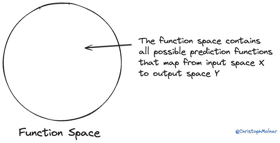
Let’s look at statistical modeling through the lens of functions. Once we have decided on a set of features X, and the target Y, we have, in theory, the entire function space f: X → Y at our disposal.

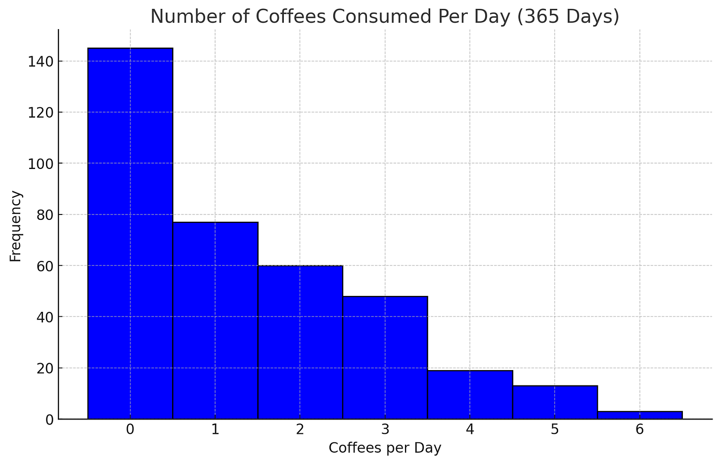
Let’s stay with the coffee example. A Poisson distribution is a typical choice for count data. However, the statistician discovers an unusual amount of zeroes.

The statistician decides on a zero-inflated Poisson regression model. That’s two models, a Bernoulli model of whether or not you will drink coffee at all. And for the days when you drink coffee, a Poisson model. This is the likelihood:

\(L(\pi,\lambda, y) = \prod_{i=1}^n\left[I(y_i=0) \left(\pi_i + (1 - \pi_i)exp(-\lambda_i)\right)+ I(y_i > 0)\left((1 - \pi_i) \frac{exp(-\lambda_i)\lambda_i^{y_i}}{y_i!}\right)\right]\)

It’s a mixture of two distributions controlled by two parameters: π, the probability of getting a zero coffee day, and λ, the number of coffees per day for coffee days.

In terms of the function space, it means we impose a smaller hypothesis space in which only models live that are compatible with a zero-inflated Poisson distribution. We can see this as a restriction bias.

Now finding a prediction model has become easier: We don’t have to look in this entire function space, but we can search in the smaller hypothesis space of zero-inflated Poissons.

We can turn the likelihood into a loss function by taking the negative logarithm of it. In fact, we can turn any likelihood into a loss function, by simply taking the negative log-likelihood. If you want to read more about this link between distributions and loss functions, see my other post:

Bridging the Gap: From Statistical Distributions to Machine Learning Loss Functions

To link the parameters to the features (day of the week, on holidays Y/N, sick Y/N, …), we could use a neural network with two outputs, one for λ, and one for π. Then we could let gradient descent do its thing.

But in classic statistical modeling, we wouldn’t use a neural network. Instead, we make stronger assumptions:

Parameterization shrinks the hypothesis space

In the zero-inflated Poisson regression, we would also say that the intensity parameter λ is the exponent of a linear function of the features:

\(\lambda_i = exp(\beta_0 + \beta_1x_{1i} + \beta_2 x_{2i} + \ldots + \beta_k x_{ki})\)

The π from the Bernoulli model would be a classic logistic model:

\(\pi = \frac{exp(\alpha_0 + \alpha_1 x_{1i} + \alpha_2 x_{2i} + \ldots \alpha_m x_{mi})}{1 + exp(\alpha_0 + \alpha_1 x_{1i} + \alpha_2 x_{2i} + \ldots \alpha_m x_{mi})}\)

Both models might potentially use different features, that’s why you see different indicators here.

This parameterization is done for multiple reasons: To make the parameters interpretable + to make estimation easier + to allow inference of the parameters. By having one parameter per feature (or rather two), we can understand them as the effects of the features on the target. We also get confidence intervals and so on.

However, we can also see it in a different light. Imposing this structure on pi and lambda further restricts the hypothesis space:

All these assumptions in statistical modeling can be seen as inductive biases. These inductive biases are designed to allow statistical inference and to make the models interpretable. Compared to the inductive biases of learning algorithms like xgboost, these biases are specifically designed, well-studied, and well-understood. The flip side is that these biases are extremely restrictive on the hypothesis space. Modeling lambda and pi with a neural network would also have carried restrictive and preferential biases. However, the restrictions would typically be less strong compared to the classic zero-inflated Poisson regression.

Inductive biases and the hypothesis space are useful mental images to think about different modeling approaches and, at least for me, also shed new light on statistical modeling. This post also emphasized that classic statistical modeling and machine learning are very different mindsets, as I describe in my book Modeling Mindsets.

Next week, we will talk about using inductive biases to your advantage.

1. There is an entire branch of non-parametric statistics, but this emphasizes the importance of parameters for most of statistical modeling. At the core, you often find a linear model combined with transformation functions to model a distribution parameter.