How Tabular Foundation Models learn without real data

The pre-training recipe behind TFMs

This is post #4 of the Tabular Foundation Model (TFM) series (see Part 1, Part 2, and Part 3).

In this post, we take a deep dive into how TFMs like TabPFN and TabICL are pre-trained to enable in-context learning (= single forward pass without weight updates). We’ll have a look into the pre-training procedure and how the pre-training data are generated (also called the prior). This post is a bit more general about pre-training TFMs, not a particular one, but I’ll reference TabPFN and TabICL mostly.

Let’s get started.

TFMs are pre-trained on millions of tables

TFMs like TabPFN are neural networks. As such, they receive the typical training (well, pre-training): Large amounts of data are fed to the randomly initialized model; stochastic gradient descent adapts the model weights.

The way TFMs work, a single “data point” is an entire supervised ML task, aka a table with both training and test data, with features and the target. A bit confusing: while I also used the word “training data” here, it refers to the train-test split in a table, and not to the training of the TFM. From now on, training/test refers to the inside-table split unless stated otherwise.

A batch of “data points” is then, e.g., for TabPFN v2, 64 such tables. That’s 64 supervised ML tasks to “solve” per batch, and the weights of the model are updated based on how well it solves them.

The entire pre-training of, for example, TabPFN v2 is based on 2 million batches. Which comes out to ~130 million tables on which this model is pre-trained.

Alright, now that we’ve established that tables are the elementary “data points” for pre-training, let’s have a look at the loss function that is optimized.

The loss function to approximate the posterior predictive distribution

The loss used is the negative log-likelihood for the target cells in the test portion of the tables. The loss is then computed as the expectation over the prior of datasets:

\(L_{PFN} = \mathbf{E}_{((\mathbf{X}_{test}, \mathbf{y}_{test})) \cup D_{train}\sim p(D)}[-\log q_\theta(\mathbf{y}_{test}|\mathbf{X}_{test}, D_{train})]\)

Let’s take this formula apart:

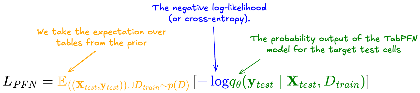
• The loss measures the negative log-likelihood of the prediction of the target test cells.

• To aggregate over the prior, we take the expectation of this negative log-likelihood across the datasets.

• p(D) is the prior over the datasets and is defined by the selection/creation of pre-training data.

• To calculate this loss for stochastic gradient descent, we can replace the expectation with the sum over the 64 datasets in the batch.

By pre-training the TFMs with this loss function, they become models that learn to approximate the predictive posterior distribution of y_test. For more details, check my post about prior-data fitted networks (PFNs).

This loss function works for both classification and regression, which are trained separately:

For classification, the architecture is hard-coded with a fixed last-layer dimension (usually 10), meaning the model is natively built for a specific maximum number of classes. If a dataset has fewer than 10 classes, the model uses the first few logits and ignores the rest during pre-training. For more than 10 classes, the model uses Hierarchical Class Extensions, grouping classes into clusters and applying the model multiple times. However, this is a trick applied at prediction-time, not during pre-training, so I might cover Hierarchical Class Extensions in a different post.

Regression, while pre-trained separately, is also treated like a classification problem: Same loss function, and the regression target is chunked into buckets (I think 100 for TabPFN v2). This turns the regression task into a classification task. By predicting the buckets, we get a probability for each and can turn this into a probability distribution for the target (the predictive posterior distribution). This gives us multiple options for the prediction: we can predict the mean, the mode, the median, or other quantiles, and even do uncertainy quantification. If interested, I could also make a longer post about TFMs for regression at some point.

TFMs are pre-trained with synthetic data

Pre-training a neural network to predict tabular data requires lots of tables to pre-train on. Interestingly, and against my intuition, many tabular foundation models are pre-trained exclusively on synthetic data. Why does it even work? Pre-training on synthetic data. I had the stance that simulating data basically means just infusing your assumptions, and what could the model possibly learn other than just reiterating these assumptions? I was very wrong on that, and now find myself very curious about pre-training on synthetic data and its implications for how data science might change in the future.

The general idea: Design a process that spits out a great variety of synthetic data on the fly, with a train and test split, targets, and features. All these synthetic datasets should show a great variety: different numbers of classes, different numbers of rows, different numbers of features, different relationships between the features and targets. So what the prior defines here is not just a sampling procedure for tables, but for full supervised machine learning tasks.

Relying on synthetic data means that TFMs don’t walk the murky path of GenAI, being trained on copyrighted material, like all the chatbots and image generators.

Anyways, how do you generate synthetic pre-training data that actually helps a model learn useful stuff so that it can do in-context learning?

Structural causal models produce pre-training data

At the heart of the prior for TabPFN (v1, v2) and TabICL is the structural causal model. Structural causal models, short SCMs, are a framework for describing causal relationships between variables and can be used to generate data.

To create a new table for pre-training, we first need to generate an SCM. On a very high level, this is how it works:

• First, sample high-level parameters of the structural causal model, like the number of features, the size of the dataset, and so on.

• Next, initiate a directed acyclic graph (DAG) that decides the relationship between features (and the target).

  • In the DAG, each node represents a variable.

  • The directed edges (arrows) represent causal influence.

• The relationship between each node and its parents (incoming arrows) is typically set as f(Pa(c)) + ε, where c is the node, Pa(c) are its parents, and f is typically a sampled modeling function.

• Not all variables (nodes) will make it into the dataset, but only a subsample will become features or targets; the others are “unobserved” variables from the perspective of the supervised ML task.

Let’s look at one example of a directed acyclic graph that instantiates parts of a structural causal model:

Directed acyclic graph describing a structural causal model.

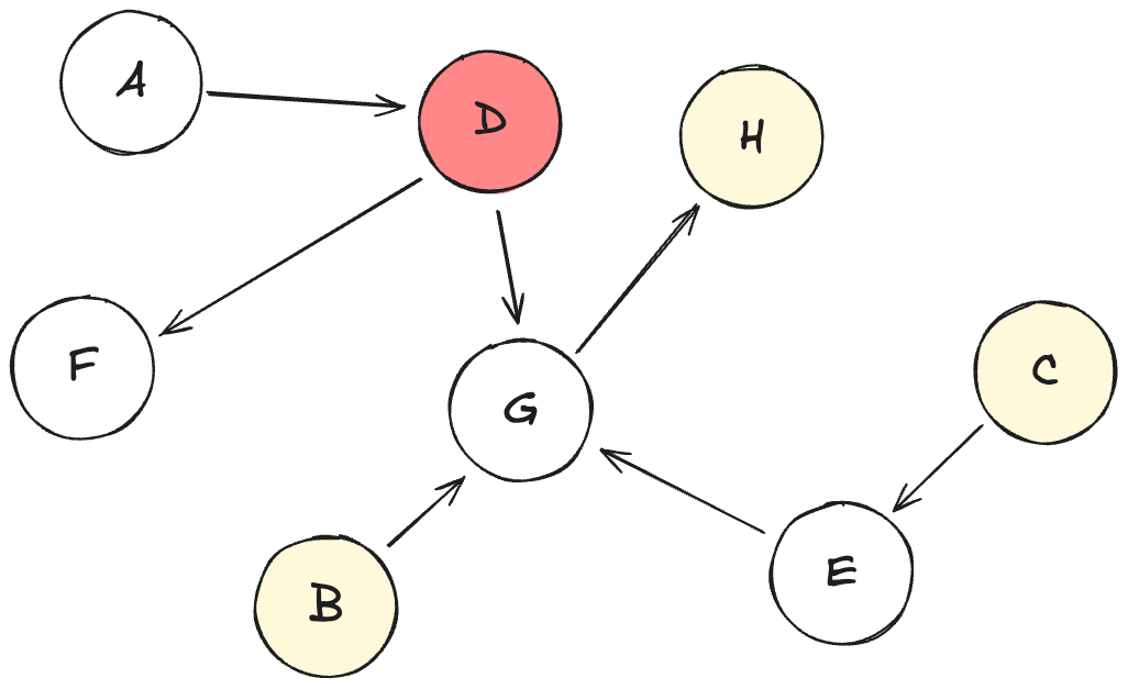
Let’s interpret this DAG:

• Each node from A to H is a variable.

• Variables have different sampled roles:

  • D is the target

  • B, C, and H are the features

  • A, E, F, G won’t make it into the data (“unobserved”)

Each dataset is sampled from an SCM

Once we have an SCM fully specified, we can sample a dataset from it. Reminder: This will later be just one “datapoint” for pre-training, so we have to repeat sampling another SCM, plus sampling from this SCM millions of times.

Here is a high-level view of how to sample a dataset from an SCM:

• Sample values for variables without parents. In the DAG above, this would be nodes: A, B, C. These are typically sampled just from Gaussian or Uniform noise.

• Then, continue propagating values through the graph, based on the relationships described by the edges: So, we would sample values for variables E and D next. These are based on sampled functions of their parent nodes, plus typically some Gaussian noise.

• Continue until all variables are sampled.

• Take all the variables that are marked as features or targets and create a table from them. Mark some of the rows as training data and the others as test data.

Like this, on the fly, you can sample SCMs from the prior, and for each SCM, sample one dataset. 64 datasets create a batch. Pre-train the model a bit more. Repeat with more batches until convergence or your GPU credits run out, or someone else needs the GPU cluster.

This overview of SCMs was very high-level. The TFMs use different ways to induce these SCMs: TabPFN v1 and TabICL use fully-connected multi-layer perceptrons (MLPs), while TabPFN v2 grows DAGs with a redirection sampling method.

The prior is the secret ingredient

With tabular foundation models, we have a new “engine” (the prior-data fitted network, PFN) that learns how to do in-context learning without any hyperparameter tuning needed to outperform Catboost and other ML algorithms on many supervised ML tasks. The fuel to the engine is the prior, the process of sampling data for pre-training.

With the design of the prior, a lot of assumptions are now poured into the model. Or rather, it decides what the model learns. Here are some of the choices that I find interesting: Structural causal models seem to work pretty well, so basing the prior on causality seems to pay off. TabICL additionally uses xgboost in the SCM edges trained on noise variables, since tree-based models seem to carry the right inductive biases for tabular data. Seems to work.

And since TFMs are neural networks, they can also be continued to be pre-trained, or fine-tuned. A few examples:

• Models like RealTabPFN v2.5 and TabDPT included real-world data in their pre-training.

• TabPFN-Wide continues pre-training on synthetic data.

• CausalFM pre-trains on causality-inspired Bayesian neural networks to handle causal inference stuff like Conditional Average Treatment Effect (CATE) estimation.

I’d expect the architecture to continuously improve over the next few years, to become faster at prediction time (they are very slow), and handle more table cells, so more features and rows.

However, when it comes to the “capabilities” of the TFM, the prior seems to be where the leverage is: You want a model that works well with your highly specific company’s tabular data? Fine-tune a TFM on your internal data. Or maybe you want a TFM that works well for data with repeated measurements? Define a data-generating process that spits out clustered data.

Prior Labs, the startup coming out of the same lab as TabPFN, seems to have identified the prior as the Moat, the competitive advantage. At least that’s my suspicion based on their decision to publish all of the code for TabPFN v2, except for the definition of the prior for generating the synthetic data.

I expect a lot of innovation in the space of tabular foundation models over the next few years. Especially innovation in the prior might become an exciting playground.