
The architecture behind TabPFN
How transformers learn from entire tables

This is the third post in the tabular foundation model (TFM) series (see part 1 and part 2).
It’s time to talk about the architecture of TabPFN (v2).
This post took me quite a while to write — the flu being one reason, but the real problem was that tabular foundation models operate on an unusual abstraction level. At least for me, who spent the last 15 years internalizing classic tabular thinking: Always seeing rows as the fundamental unit. The simple times when training data was used for model training, and test data for prediction.
TabPFN and other tabular foundation models (TFMs) do in-context learning, so at prediction time, they take in the entire dataset, combining training and testing data. At the same time, the fundamental unit on which TabPFN operates is individual cells of the table, or rather, their embedded representations. My row-based brain had a tough time understanding this, but I believe I have now wrapped my head around it. And with this post, I hope to convey the ideas in a helpful way to you.
The TabPFN library is huge. And from the papers alone, I had a hard time understanding the architecture in detail. Fortunately, there is a paper called “nanoTabPFN: A Lightweight and Educational Reimplementation of TabPFN,”1 which comes with the nanoTabPFN GitHub repository that contains a simplified implementation of TabPFN v2. Without the effort of the authors, this post would have probably taken me twice the time.
Anyways. Let’s start.
Table cells become computational units
To understand the architecture, you need to understand the fundamental unit on which TabPFN models operate. TabPFN and other TFMs use the transformer, which was designed for token-based sequential data (text). Like this:

In large language models, these tokenized texts get embedded, meaning each token (= sub-word) is represented by a vector. Transformer-based architectures then operate on these vectorized representations of the tokens. The so-called attention mechanism acts as a way of querying the input tokens for predicting the output tokens.
Tables don’t contain tokens. They contain scalars. However, to apply the transformer to tables, we need to rethink tables. For TabPFN, these fundamental units are the table cells (feature=value or target=value) on which computations are done.
")
TabPFN is an encoder-decoder transformer
TabPFN and many other TFMs follow an encoder-decoder transformer architecture. This means it has the following high-level structure:
The encoder pre-processes the table cells and embeds them (both features and target, and training and test).
Multiple, sequential transformer layers take the embeddings of each table cell and repeatedly enrich them with the help of data-point-wise and feature-wise attention.
The decoder maps the high-dimensional embedding back to actual values to predict the test data (which are just a subset of the cells).
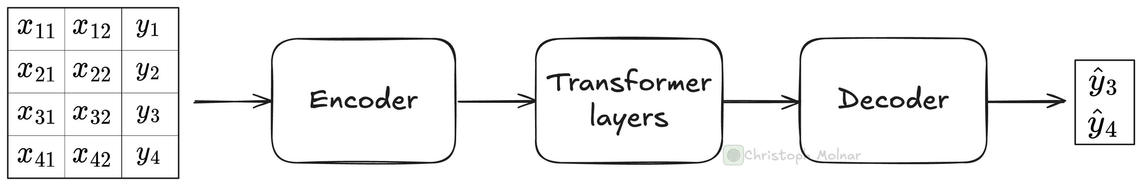
We start with an NxP table, where N is the number of rows in the table (combined train and test), and P is the number of features. After the encoding, the data is (conceptually) represented by an NxPxE Tensor, where E is the embedding length. With each transformer step, the NxPxE structure is retained, but with updated and enriched embeddings for each cell. The decoder maps the NxPxE Tensor to a Tensor of size N_testxO, where N_test is the number of test data points, and O is the output dimension.
Keep that high-level view in mind while we dig deeper into the individual parts, starting with the encoder.
The encoder pre-processes and embeds
In a single forward pass, we push the entire combined training and test data with features and targets down the neural network.
The first step is the pre-processing and embeddings, which work differently for feature and target cells.
The feature encoder pre-processes and embeds feature cells:
All features are normalized, based on the training data’s mean and standard deviation: (x-mean)/std.
After normalization, values below -100 and above 100 are clipped.
The features are linearly embedded. Before embedding, a cell’s value is a scalar. During embedding, a weight vector with length embedding size E (512 for TabPFN and 96 for nanoTabPFN) is multiplied with each scalar, and a bias is added, producing an E-length embedding vector for each cell. The weights are the same for all feature cells.
The target encoder only does two things:
The test values (y_test) are filled in with the mean of the target in the training data (mean(y_train)). This isn’t for imputation, but rather for providing a starting value.
The target values are also linearly embedded, but with a weight vector different from the linear feature embedding.
nanoTabPFN has no positional embedding. However, TabPFN has a version of positional embedding for the features (not the target): After the linear embedding, the encoder adds a random vector to the cells of each feature. This random vector is constructed via a projection, part learned, part random. The positional embedding helps TabPFN better distinguish between the features.
After encoding, cells no longer contain scalars, but vectors. The transformer layers operate on these vector representations.
The transformer layers route and aggregate information
The main computations happen within the transformer layers, which contain two attention layers: feature attention and datapoint attention. If you are not familiar with the transformer and attention, I can recommend this blog post.
The attention mechanism calculates dynamic weights for different parts of an input sequence, allowing the model to focus on the most relevant features regardless of their distance from each other.
TabPFN contains multiple transformer layers in sequence. Here is what a single transformer layer looks like:
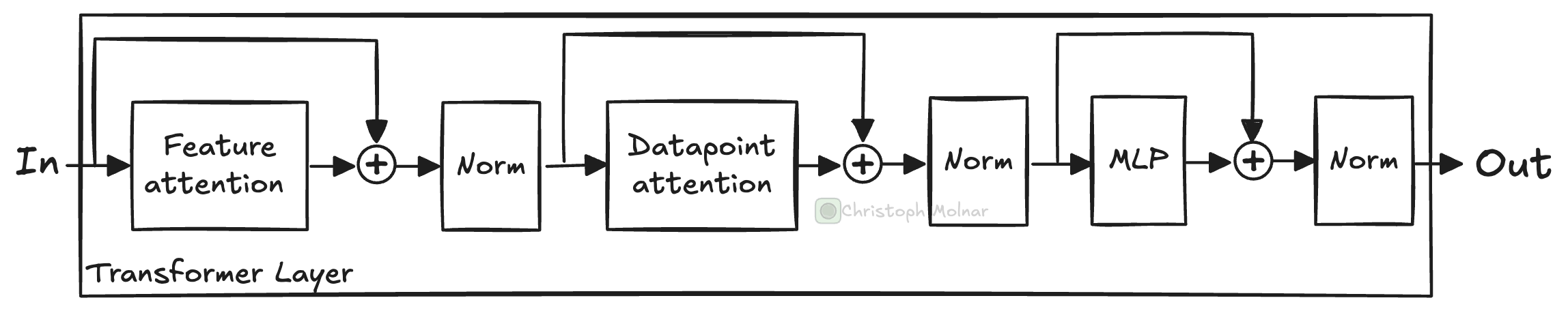
A transformer layer in nanoTabPFN contains the following elements:
Feature attention: Attention mechanism that attends to cells in the same row.
Datapoint attention: Attention mechanism that attends to cells in the same column.
Multi-layer perceptron (MLP): A fully-connected network with 2 layers.
Layer norm: After each operation, the cell representations are normalized.
Skip connections, also called residual layers, before attention and MLP blocks.
The most exciting parts are the two attention mechanisms.
Feature attention allows attending to other cells in the same row, meaning from the same data point. After this attention step, each cell’s vector representation is changed by the information contained in other cells of that same row (= same data point). In this step, the model can share information between all the features, including the target.
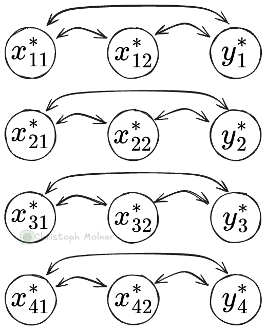
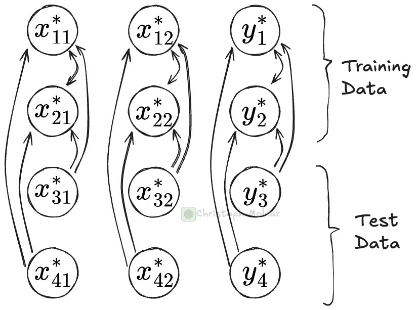
Datapoint attention attends to cells from other data points. So if you look at the vector representation for, say, cell x_12 (row 1, column 2), the datapoint attention layer can attend to other cells in the same column (and itself), for example, to x_22. This is somewhat similar to soft k-nearest neighbors: It finds the closest neighbor cells (from the same column) and pulls in some of their information. Datapoint attention distinguishes via masking whether a cell is from training or test data: Cells can only attend to training data cells, but not to test data cells.
While the attention mechanisms are busy moving around information between cells, what the heck is the multi-layer perceptron (MLP) doing? The MLP consists of two fully-connected linear layers with a GELU activation function in between. The MLP acts as the primary processing unit for the information from the attention mechanisms and also introduces the needed non-linearity to model more complex functions. While both attention-mechanisms pull in information, the MLP takes in the embedding of a cell and can update the representation.
The transformer layer is repeated, sequentially, a few times. Each time, the input to the next transformer is based on the output of the previous. Each iteration routes and aggregates information in the table. If TabPFN is anything like convolutional neural networks, I would expect that with each transformer iteration, the model builds up more and more abstract representations of the tabular cells. TabPFN has 12 transformer layers, while nanoTabPFN has 3.
After the transformer layers, we have an enriched representation of our tabular dataset. But we wanted to know y_test, so we need to decode this representation.
The decoder predicts the test data
The decoder takes as input all the embeddings of cells that represent the test targets (y_test), which, after the transformer layers, are now enriched representations containing information from other cells as well. These vectors are pushed through a multi-layer perceptron: two-linear layers with GELU activation. Thereby, the same MLP is applied to each y_test cell individually to decode the representation into a prediction.
For classification, the result is then pushed through a softmax layer, which for classification is fixed to 10 outputs.
In short, during in-context learning for tabular models, the model treats the training data as a “dynamic lookup table”, routes information around the cells, and aggregates it, building up more and more abstract knowledge about the cell values.
See you next week
That’s it for today. Quite a lot to digest. Keep in mind that this was about nanoTabPFN. TabPFN is more complex since it uses some tricks like feature grouping, adding random embeddings, and row hashing. Other TFMs, like TabICL, again have differences in their architectures.
Next week, we’ll go into details of the training, which I am quite excited about since it’s about creating millions of synthetic data-generating processes. By the way, let me know in the comments if you have questions about TFMs, so I know what to focus on.
Pfefferle, Alexander, et al. “nanoTabPFN: A Lightweight and Educational Reimplementation of TabPFN.” arXiv preprint arXiv:2511.03634 (2025).
Am I missing something when you talk about: ‘Datapoint attention attends to cells from other data points. So if you look at the vector representation for, say, cell x_12 (column 1, row 2),’. … don’t you mean row 1, column 2?
This article is phenomenal by the way. Thank you!
Thanks for the writeup. Wanted to point out something -- it's a bit confusing to call this an "encoder-decoder" architecture. When people say that about transformers, they are usually referring to two transformer stacks that handle sequences differently. TabPFN is an encoder-only transformer, with *feature* and *output* encoder/decoder, not to be confused with how T5 is an encoder-decoder.