Week #2: Intuition Behind Conformal Prediction
The surprisingly simple recipe that underpins this universal uncertainty quantification method
Reading time: 8 min
Welcome to course week #2 of Introduction to Conformal Prediction (see #1).
This week, we’ll learn:
how conformal prediction works on an intuitive level
the general “recipe” that most conformal prediction algorithms follow
parallels to model evaluation
Intuition Behind CP
Last week we focused on code and a use case of for conformal prediction for classification. This time, we look at how conformal prediction works on an intuitive level.
Let’s say you have an image classifier that outputs probabilities but you want prediction sets with a guaranteed coverage of the true class.
Conformal prediction for classification works the same for tabular and image classification, because the algorithm only works with the model outputs.
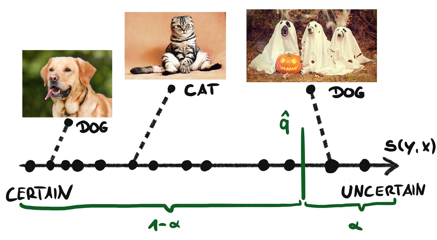
We first sort the predictions of the calibration dataset from certain to uncertain. The calibration dataset must be separate from the training dataset. For the image classifier, we could use as so-called non-conformity score s_i = 1 - f(x_i)[y_i] where f(x_i)[y_i]is the model output for the true class. This procedure places all images somewhere on the scale of uncertainty, like in the following figure.
The dog on the left could have 95% model output, therefore getting s = 0.05, but the dogs on the right in their spooky costumes could bamboozle the neural network. This spooky image gets a score of only 15% for class dog translating into a score of s = 0.85.
We rely on this ordering of the images to divide the images into certain (or conformal) and uncertain. How big each portion is, depends on the confidence level α that the user picks.
If α = 0.1, then we want to have 90% of the non-conformity scores in the “certain” section. Finding the threshold is easy because it means computing the quantile q: the score value where 90% of images are below and 10% are above:
In this example, the spooky dogs fall into the uncertain region.
But that’s the point where I was confused for some time: We picked the threshold without looking at wrong classifications. Because there will be scores for wrong classes that also fall into the “certain” region, but we seemingly ignore them when picking the threshold q.
I came to the conclusion that, within the prediction sets, conformal prediction foremost controls the coverage of positive labels: there’s a guarantee that 1- α of the sets contain the true class.
So is it really true that negative examples don’t matter? Because this would mean that we don’t care how many wrong classes are in the prediction sets. If we didn’t care about false positives at all, we could always include all the classes in the prediction sets and guarantee coverage of 100%! A meaningless solution, of course.
So one part of conformal is controlling the coverage of positive labels and the other part is minimizing negative labels, meaning not having too many “wrong” labels in the prediction sets.
CP researchers therefore always look at the average size of prediction sets. Given that two CP algorithms provide the same guaranteed coverage, the preferred algorithm is the one that produces smaller prediction sets. In addition, some CP algorithms guarantee upper bounds on the coverage probability, which also reduces the risk of “let’s just include all classes”.
Let’s move on to the conformal prediction step.
For a new image, we check all possible classes. Each possible class for an image gets a non-conformity score that can either fall below or above the threshold q.
All scores below the threshold are conformal with scores that we observed in the calibration set and are seen as certain enough (based on α). These classes form our prediction set.
In this example, the image has the prediction set {cat, lion} because both classes are “conformal” and made the cut. All other class labels are too uncertain and therefore excluded.
Now perhaps it is clearer what happens to the "wrong classes": If the model is worth its money, the probabilities for the wrong classes will be rather low. Therefore the score will probably be above the threshold and the corresponding classes will not be included in the prediction set.
One Recipe With Different Implementations
Conformal prediction for classification is different from CP for regression. For example, we use different non-conformity scores and conformal classification produces prediction sets while conformal regression produces prediction intervals. Even among classification, there are many different CP algorithms.
All conformal prediction algorithms follow roughly the same recipe. That’s great as it makes it easier to learn new CP algorithms.
Conformal prediction has 3 steps: training, calibration, and prediction.
Training is what you would expect:
Split data into training and calibration
Train model on training data
Calibration is where the magic happens:
Compute uncertainty scores (aka non-conformity scores) for calibration data
Sort the scores from certain to uncertain
Decide on a confidence level α (α=0.1 means 90% coverage)
Find the quantile q where 1-α (multiplied with a finite sample correction) of non-conformity scores are smaller
Prediction is how you use the calibrated scores:
Compute the non-conformity scores for the new data
Pick all y’s that produce a score below q
These y’s form your prediction set or interval
In the case of classification, the y’s are classes and for regression, the y’s are all possible values that could be predicted.
A big differentiator between conformal prediction algorithms is the choice of the score. In addition, they can differ in the details of the recipe and slightly deviate from it as well.
In one way, the recipe isn’t accurate, or rather it’s about a specific version of conformal prediction that is called split conformal prediction.
Splitting the data once into training and calibration is not the best use of data. If you are familiar with evaluation in machine learning, you won’t be surprised about the following extensions.
Parallels To Out-Of-Sample Evaluation
So far we have learned about conformal prediction using a single split into training and calibration. But you can also do the split repeatedly using:
k-fold cross-splitting (like in cross-validation)
bootstrapping
jackknife
Do these sound familiar to you? If you are familiar with evaluating and tuning machine learning algorithms, then you already know these resampling strategies.
For evaluating or tuning machine learning models, you also have to work with data that was not used for model training. So it makes sense that we encounter the same options for conformal prediction where we also have to find a balance between training the model with as much data as possible, but also having access to “fresh” data for calibration.
For cross-conformal prediction, you split the data, for example, into 10 pieces. You take the first 9 pieces together to train the model and compute the non-conformity scores for the remaining 1/10th. You repeat this step 9 times so that each piece is once in the calibration set. You end up with non-conformity scores for the entire data set and can continue with computing the quantile for conformal prediction.
If you take cross-conformal prediction to the extreme you end up with the jackknife method (also called leave-one-out) where you train a total of n models, each with n-1 data points.
All three options are inductive approaches to conformal prediction. Another approach is transductive or full conformal prediction. It’s a computationally costly approach as transductive CP requires retraining the model for every new data point in combination with every possible y. I won’t cover transductive conformal prediction in this course.
Which approach should you pick?
Single split: Computation-wise the cheapest. Results in a higher variance of the prediction sets and non-optimal use of data. Ignores variance from model refits. Preferable if refitting the model is expensive.
jackknife: Most expensive, since you have to train n models. The jackknife approach potentially produces smaller prediction sets/intervals as models are usually more stable when trained with more data points. Preferable if model refit is fast and/or the dataset is small.
CV and other resampling methods: balance between single split and jackknife.
In the MAPIE Python library, switching between resampling techniques is as simple as changing a parameter:
cp = MapieRegressor(model, cv="prefit")The code above uses the split strategy, but with a single change it uses cross-splitting:
cp = MapieRegressor(model, cv=10)MAPIE really is a convenient library. Give it a try.
How does conformal prediction integrate with training/validation/testing in machine learning?
So far I haven’t found a recommendation, but here is my current view: the final performance evaluation and calibration should be doable with the same data and therefore calibration and testing datasets could be the same. Both calibration and evaluation shouldn’t impact modeling choices and therefore not interfere with each other. Please comment if you think there’s a problem with this approach.
For the rest of the course, we will mostly talk about split versions of the conformal prediction algorithms, as these are simpler to introduce.
That’s a wrap for this week. Next week we will have a look at conformal prediction for regression where we turn predictions into prediction intervals.
Book Announcement 📓
I’m working on an introductory book for conformal prediction!
The book will be an extension of this course with more in-depth explanations, full code examples in Python, and additional topics not covered in this course.
I will keep you posted about the progress of the book. Are you interested to be a Beta reader of the book? Just send me a quick email.
What To Do Next
Take a few minutes and try to formulate how conformal prediction works on an intuitive level. If questions come up, feel free to leave them as comments here and I’ll try to help you.
If you are not signed up for this newsletter, subscribe to get the rest of this email course:
Check out my book on Conformal Prediction which provides hands-on examples to quantify uncertainty in your application!


Keeping calibration and test sets different is usually a good idea, as otherwise the model will be peeking into the test set during the calibration stage. In the research papers we have always kept them separate.
Thanks Christoph for this series!.
Do you plan to use R also?.
In R, there are several packges for conformal analysis most of them for regression.
And just one for classification (conformalClassification), but for "randomForest" models.
Thanks,
Carlos.