Week #3: Conformal Prediction For Regression
Two approaches that give you prediction intervals
Reading time: 8 min
Welcome to week #3 of the course Introduction to Conformal Prediction (see #1, #2)
This week we will look at conformal prediction for regression. In detail you will learn:
How to turn point predictions into prediction intervals
How to conformalize quantile regression
Conformal Prediction For Regression
In regression, the target is on a continuous scale, unlike in classification where the goal is to predict distinct classes. If the L2 loss was used for training the regression model, the prediction of the model can be interpreted as the conditional mean of the target:
But even if other losses were used, the prediction is a point prediction.
With conformal prediction, we can turn this point prediction into a prediction interval that comes with a guarantee of covering the true class in future observations. These types of intervals aren’t new. Quantile regression, for example, can have the same goal, but usually doesn’t come with the guarantees of conformal regression.
This gives us two starting points for creating a prediction interval:
start from a point prediction
start from (non-conformal) intervals produced by quantile regression
We will try out both approaches for predicting rents.
Rent Index
Let’s predict rents from *checks notes* 2003. The year doesn’t really matter except to make everyone sad that rents have gone up so much. What matters is the use case: the data was collected for computing a rent index.
A rent index defines acceptable rents per square meter based on the properties of the apartment such as location, size, and equipment. In Germany, landlords are required to adhere to such a rent index.
The rent index is modeled using generalized additive models as there is a requirement for the model to be interpretable. But we will use a random forest and gradient boosting.
It’s a perfect use case for conformal prediction because we are not only interested in the mean prediction, but in a range of acceptable rents per square meter. The uncertainty in the rent comes from remaining market uncertainties, lack of some features e.g. due to legal reasons, and of course imperfections of the model.
Conformalized Mean Regression
In this version, we start with a Random Forest for the regression model, where we predict the rent per square meter given all the features. Using conformal prediction we will turn the point prediction into a prediction interval.
Conformalized Mean Regression in MAPIE
I trained the Random Forest with sklearn (RandomForestClassifier). Again we can use the MAPIE library for conformalizing the model. As ɑ we pick 0.33 so that 2/3 of the true rents are covered by the intervals in expectation.
mapie_reg = MapieRegressor(estimator=model, cv="prefit")
mapie_reg.fit(X_calib, y_calib)
y_pred, y_cis = mapie_reg.predict(X_new, alpha=1/3)
The first apartment in X_new has a size of 117 square meters. It gets the prediction of 5.93 EUR per square meter (so cheap), with a 2/3 prediction interval of [3.8; 8.0].
If we multiply that by the area, the predicted rent of the apartment is 694 EUR, while the actual rent for this data point is 555 EUR. If we multiply the confidence interval for the prediction with the square meters, we get an interval of [446 EUR, 940 EUR].
How does the rent per square meter depend on the area?
We can visualize the prediction intervals by feature “area”:

The larger the area, the less rent, which makes sense as the target is the rent per square meter, not the total rent.
Are you wondering why the prediction intervals look like they were colored in by a 5-year-old?
There’s no guarantee that two points with similar areas have similar predictions since they usually differ in many other features. If you were looking for a plot that only shows the effect of 1 feature, you should look into Partial Dependence Plots and Accumulated Local Effect Plots.
But if you look into tutorials, you usually get these nice-looking intervals and that’s because they only use 1 feature. This practice sets unrealistic beauty standards for plots of prediction intervals and has to stop.
Theory
Using MAPIE, turning a regression model into a conformal predictor is simple, but how does it work in theory?
Good news: It’s in most parts the same conformal prediction recipe that we used also in classification:
Split data into training and calibration
Train model on training data
Compute non-conformity scores
Find threshold q
Form prediction intervals for new data
The main difference between classification and regression is the non-conformity score that we use:
This function, when using the true y, computes the absolute residual of the prediction. Conformalizing this score means finding where to cut off so that 1-ɑ of the predictions have a score below and ɑ a score above. In our rent index case, this value is q=1.97. This means that all intervals have a width of 2 * 1.97 = 3.94.
To compute the prediction interval for a new data point, we include all possible y’s that produce a score below q.
This procedure treats both directions equally and isn’t adaptive to different regions of the feature space. But we can get adaptive intervals with these options/alternatives:
Instead of a single split, we could use cross-splitting or leave-one-out (jackknife). By doing so the intervals become slightly adaptive due to the refitting.
Adaptive conformal regression: Instead of using residuals, we use standardized residuals. This approach requires a second model to estimate the variance and scale the residuals:
\(s(y, x) = \frac{|y - \hat{f}(x)|}{\hat{\sigma}(x)}\)Another adaptive approach is quantile regression which we discuss next.
Conformalized Quantile Regression
The other option is to start with quantile regression. That means that you already have one or two models that give you the lower and upper quantiles of rent per square meter for an apartment.
Quantile regression can already produce prediction intervals, but we have no formal guarantees that the coverage is correct. For example, the interval from the 1/6-quantile to the 5/6-quantile may or may not actually contain 2/3 of the data.
We can use conformal prediction to guarantee coverage.
Theory
Conformalized quantile regression relies on the same general conformal prediction recipe as other conformal predictors, but with a score that matches the task:
The score is positive if the true value y lies outside of the interval, and negative if it lies inside.

The threshold q can be interpreted as the term by which the interval has to be expanded (on both ends) or shortened. If 1-ɑ of the y’s are already within the interval (meaning the model is well calibrated), then the threshold would be at 0. A positive threshold means that the original intervals were too narrow, and a negative one that quantile intervals were too wide.
To compute the prediction interval, we add the threshold to the upper bound and subtract it from the lower bound (aka the old quantiles).
The calibration part of the procedure is not adaptive, since the same term will be added no matter the feature values. However, the entire procedure is adaptive since quantile regression is adaptive.
Conformalized Quantile Regression in MAPIE
In MAPIE you need three outputs: median, lower and upper quantiles. The median is not used for anything, MAPIE just returns it back to you.
First, we train a quantile regression model, in this case with gradient boosting. Other options would be linear quantile regression or quantile forests. Furthermore, we could use the pinball loss and train any model that accepts arbitrary loss functions.
Training the gradient boosting models in sklearn is simple:
low = GradientBoostingRegressor(loss='quantile',alpha=1/6)
median = GradientBoostingRegressor(loss='quantile',alpha=0.5)
up = GradientBoostingRegressor(loss='quantile',alpha=5/6)
In addition, you have to fit the models, which I omitted here. We use MAPIE for conformalizing the model. And yet again, it’s a smooth experience:
cqr = MapieQuantileRegressor([low, median, up], alpha=[1/6, 0.5, 5/6],    cv="prefit")
cqr.fit(X_calib, y_calib)
cqr.predict(X_new)
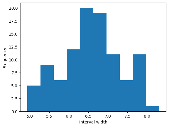
Looking at the interval widths, we can see that the intervals are indeed of different sizes:
At one point I said conformal prediction turns point predictions into prediction sets/intervals. While that’s still true, the statement cuts too short since this quantile regression approach shows that it can also formalize output that is already an interval.
And that’s it for this week. Next week we’ll get an overview of conformal prediction algorithms.
Last week’s discussion: test vs calibration
Last week, there was an interesting discussion on whether or not to use the same dataset for calibration and performance evaluation. Valeriy mentioned that he and other researchers usually separate both.
If you evaluate the performance of the calibrated model, you need fresh data. In this case, calibration and testing have to be different data or otherwise you will spoil the performance evaluation.
If you want to be on the safe side and if you have enough data, I would recommend keeping calibration and test data separated.
I still believe you might be able to use the calibration set to evaluate the original, non-conformal model output, as long as it doesn’t influence any modeling decisions. But take it with a grain of salt.
Further Resources
Are you ready to dive deeper?
Read chapters 2.2 and 2.3 of the Gentle Introduction paper
Read the paper Conformalized Quantile Regression which also gives an overview of all other approaches that start with point prediction models.
Check out the MAPIE documentation on regression which has an extensive comparison of different splitting strategies, from simple split to different versions of leave-one-out (jackknife).
Course Outline
Check out my book on Conformal Prediction which provides hands-on examples to quantify uncertainty in your application!


an annoying thing in this context is that you can't run quantile regressions in XGBoost (at least not from what I can gather,) so you'd either have to change to another gradient boosting model (easier said than done if you're in production) or run the former approach.
Interesting piece! In the context of using conformal predictions to calibrate coverage for a quantile regression forecaster, I’ve always found it a bit unsettling that a poorly performing model can still achieve seemingly "accurate" coverage - simply by applying conformal correction terms. Doesn't that defeat the purpose of having a well-calibrated forecaster in the first place?
I wonder what your thoughts are on this. To me, conformal prediction should be seen less as a fix and more as a diagnostic tool. If you need large correction terms, it likely signals that your model isn’t learning the underlying relationships well. In that sense, conformal methods might be better suited as a sanity check on your quantile forecaster model, rather than a blanket solution for coverage calibration.
Curious how this is used in real-world deployments - do practitioners rely on conformal corrections as a crutch, or do they use them to flag deeper issues in the modeling pipeline?